Fractional Transforms in Optical Information Processing
Tatiana Alieva
Facultad de Ciencias F´ısicas, Universidad Complutense de Madrid, Ciudad Universitaria, 28040 Madrid, Spain Email:[email protected]
Martin J. Bastiaans
Faculteit Elektrotechniek, Technische Universiteit Eindhoven, Postbus 513, 5600 MB Eindhoven, The Netherlands Email:[email protected]
Maria Luisa Calvo
Facultad de Ciencias F´ısicas, Universidad Complutense de Madrid, Ciudad Universitaria, 28040 Madrid, Spain Email:[email protected]
Received 31 March 2004
We review the progress achieved in optical information processing during the last decade by applying fractional linear integral transforms. The fractional Fourier transform and its applications for phase retrieval, beam characterization, space-variant pattern recognition, adaptive filter design, encryption, watermarking, and so forth is discussed in detail. A general algorithm for the fractionalization of linear cyclic integral transforms is introduced and it is shown that they can be fractionalized in an infinite number of ways. Basic properties of fractional cyclic transforms are considered. The implementation of some fractional transforms in optics, such as fractional Hankel, sine, cosine, Hartley, and Hilbert transforms, is discussed. New horizons of the application of fractional transforms for optical information processing are underlined.
Keywords and phrases:fractional Fourier transform, fractional convolution, fractional cyclic transforms, fractional optics.
1. INTRODUCTION
During the last decades, optics is playing an increasingly im-portant role in computing technology: data storage (CD-ROM) and data communication (optical fibres). In the area of information processing, optics also has certain advantages with respect to electronic computing, thanks to its massive parallelism, operating with continuous data, and so forth [1,2,3]. Moreover, the modern trend from binary logic to fuzzy logic, which is now used in several areas of science and technology such as control and security systems, robotic vi-sion, industrial inspection, and so forth, opens up new per-spectives for optical information processing. Indeed, typical optical phenomena such as diffraction and interference in-herit fuzziness and therefore permit an optical implementa-tion of fuzzy logic [4].
The first and highly successful configuration for opti-cal data processing—the optiopti-cal correlator—was introduced by Van der Lugt more than 30 years ago [5]. It is based on
This is an open access article distributed under the Creative Commons Attribution License, which permits unrestricted use, distribution, and reproduction in any medium, provided the original work is properly cited.
the ability of a thin lens to produce the two-dimensional Fourier transform (FT) of an image in its back focal plane. This invention led to further creation of a great variety of optical and optoelectronic processors such as joint correla-tors, adaptive filters, optical differentiators, and so forth [6]. More sophisticated tools such as wavelet transforms [7] and bilinear distributions [8,9,10,11,12,13,14], which are ac-tively used in digital data processing, have been implemented in optics.
space-variant filtering [29,57,58,59,60,61,62,63,64,65, 66,67, 68, 69, 70, 71, 72, 73, 74, 75, 76, 77], encryption [78,79,80,81,82,83,84,85], watermarking [86,87], cre-ation of neural networks [88,89,90,91,92,93], and so forth, while the fractional Hilbert transform was found to be very promising for selective edge detection [94,95,96]. Several fractional transforms can be performed by simple optical configurations.
In this paper, we review the progress achieved in opti-cal information processing during the last decade by appli-cation of fractional transforms. We will start from the defi-nition of a fractional transformation inSection 2. Then we consider, in Section 3, the fractionalization in paraxial op-tics described by the canonical integral transformation. Two fractional canonical transforms, the Fresnel transform and the fractional FT, are commonly used in optical information processing. The fractional FT, which is a generalization of the ordinary FT with an additional parameterαthat can be in-terpreted as a rotational angle in phase space, is considered in more detail.
Since the convolution operation is fundamental in in-formation processing, there were several proposals to gen-eralize it to the fractional case. InSection 4, we define the generalized fractional convolution, and in Sections5–8, we consider its application for information processing: phase re-trieval, signal characterization, filtering, noise reduction, en-cryption, and watermarking.
The second part of the paper will be devoted to the frac-tionalization procedure of other important transforms. We will restrict ourselves to the consideration of cyclic trans-forms, which produce the identity transform when they act an integer number of timesN. In Sections9–11, we will show that there are different ways for the construction of a frac-tional transform for a given cyclic transform. InSection 12, we briefly mention the common properties of fractional cyclic transforms.
The fractional Hankel, Hartley, sine and cosine, and Hilbert transforms, which can all be implemented in optics, will be considered inSection 13. Finally, we discuss the main lines of future development of fractional optics inSection 14 and make some conclusions.
2. FRACTIONAL TRANSFORM: A GENERAL DEFINITION
The word “fraction” is nowadays very popular in different fields of science. We recall fractional derivatives in math-ematics, fractal dimension in geometry, fractal noise, frac-tional transformations in signal processing, and so forth. In general, “fractional” means that some parameter has no longer an integer value.
To define the fractional version of a given linear integral transform, we consider the operatorRof such a transform, acting on a function f(x),
Rf(x)(u)= ∞
−∞K(x,u)f(x)dx, (1)
with K(x,u) the operator kernel. As an example we men-tion the Fourier transformamen-tion, for which the kernel reads
K(x,u) = exp(−i2πux). The fractional transform operator is denoted byRp, where pis the parameter of fractionaliza-tion:
Rpf(x)(u)= ∞
−∞K(p,x,u)f(x)dx. (2) We will formulate some desirable properties of this fractional transform first.
The fractional transform has to be continuous for any real value of the parameter p, and additive with respect to this parameter: Rp1+p2 = Rp2Rp1. Moreover it has to
re-produce the ordinary transform and powers of it for integer values of p. In particular, for p =1 we should get the ordi-nary transformR1 =R, and for p =0 the identity trans-form R0 = I. From the additivity property it follows that ∞
−∞K(p1,x,u)K(p2,u,y)du=K(p1+p2,x,y). Note that the parameterp, as we will see further, may be given by a matrix, and the additivity property is then formulated easily as the product of the corresponding matrices.
As we have mentioned in the introduction, some frac-tional transforms arise under consideration of different problems: description of paraxial diffraction in free space and in a quadratic refractive index medium, resolution of the nonstationary Schr¨odinger equation in quantum mechanics, phase retrieval, and so forth. Other fractional transforms can be constructed for their own sake, even if their direct ap-plication may not be obvious yet. In particular, inSection 9 we consider a general algorithm for the fractionalization of a given linear cyclic integral transform. The application of a particular fractional transform for optical information pro-cessing then depends on its properties and on the possibility of its experimental realization in optics.
3. FRACTIONALIZATION IN PARAXIAL OPTICS: THE CANONICAL INTEGRAL TRANSFORM
Analog optical signal processing systems are often described in the framework of paraxial scalar diffraction theory. A typ-ical subset of such a system is displayed inFigure 1and con-tains a thin lens with focal distance f, preceded and followed by two sections of free space with distances z1 andz2, re-spectively. Note that the conventional Van der Lugt correla-tor [5,6], mentioned in the introduction, is constructed by a cascade of two such subsets, with each subset forming an FT system (z1=z2= f) and with a filter mask inserted between them. A monochromatic optical field in a transversal plane (x,y) is then described either by a complex field amplitude
f(x,y) for the coherent case, or by the two-point correla-tion funccorrela-tionΓ(x1,x2;y1,y2)= f(x1,y1)f∗(x2,y2)for the partially coherent case, where the asterisk denotes complex conjugation and·indicates ensemble averaging; note that these cases correspond to a deterministic or a stochastic sig-nal description in sigsig-nal theory, respectively.
Input Output z1 z2
f
Figure1: A typical optical information processing system.
setup depicted in Figure 1 and the complex amplitude
FM(xout,yout) at the output plane of it are related by the input-output relationship [97]
FM
xout,yout
=RMfx in,yin
xout,yout
= ∞
−∞ ∞
−∞KMx
xin,xout
KMy
yin,yout
×fxin,yin
dxind yin,
(3)
where the kernelKMx(xin,xout) takes the form
KMx
xin,xout = 1 ibx exp
iπaxx
2
in+dxxout2 −2xoutxin
bx
, bx=0,
1
ax exp
iπcxx
2 out ax δ
xin−xout
ax
, bx=0,
(4)
with
Mx=
ax bx
cx dx =
1−z2
fx λ
z1+z2−z1z2
fx
− 1
λ fx
1−z1
fx (5)
andλthe optical wavelength, and where similar expressions, withxreplaced byy, hold for the kernelKMy(yin,yout) and
the matrixMy. Note that the optical wavelengthλenters the expressions forb andcas a mere scaling factor; very often, we like to work with reduced, dimensionless coordinates, in which casebandctake a form that would also be achieved by assigning an appropriate value toλ. We remark that the application of cylindrical lenses, fx= fy, permits to perform anamorphic transformations.
The coefficientsax,bx,cx, anddx that arise in the ker-nel (4), are entries of the general, symplectic ray transforma-tion matrix [98] that relates the position (x,y) and direction (ξ,η) of an optical ray in the input and the output plane of a so-called first-order optical system, and we have
xout ξout =
ax bx
cx dx
xin
ξin
=Mx
xin
ξin
(6)
and a similar relation for the other dimension, withxandξ
replaced by yandη, respectively. For separable systems, to which we restrict ourselves throughout, symplecticity reads simply axdx−bxcx = 1 andaydy−bycy = 1. The trans-form described by (3) is known by such names as canon-ical integral transform and generalized Fresnel transform [97,98,99,100].
Special cases of canonical integral transform systems in-clude
(i) an imaging system (1/z1+ 1/z2=1/ f, and hencead= 1 andb=0);
(ii) a simple lens (z1 =z2 =0, and hencea =d=1 and
b=0);
(iii) a section of free space (f → ∞, and hencea=d=1 andc = 0), which is also known as a parabolic sys-tem [97] and which in the paraxial approximation per-forms a Fresnel transformation;
(iv) an FT system (z1 = z2 = f, and hencea = d = 0 andbc= −1), and more generally, a fractional FT sys-tem [15,16,17,18] (z1=z2=2f sin2(α/2) [22], and hencea=d=cosαandbc= −sin2α), which is also known as an elliptic system [97]; the common case for whichb= −c=sinαfollows when we normalizex/ξ
with respect toλ fsinα, and can also be achieved by formally choosingλ fsinα=1;
(v) a hyperbolic system [97], with a = d = coshαand
bc=sinh2α.
To treat the propagation of partially coherent light through first-order optical systems, it is advantageous to describe such light not by its two-point correlation func-tionΓ(x1,x2;y1,y2) as mentioned before, but by the related Wigner distribution (WD) [101, Chapter 12]. Of course, the coherent case considered in (3) is just a special case of this more general, partially coherent case. The Wigner distribu-tion of partially coherent light is defined in terms of the two-point correlation function by
W(x,ξ;y,η)
= ∞ −∞ ∞ −∞Γ
x+x
2,x−
x
2;y+
y
2,y−
y
2
×exp−i2πξx+ηydxd y.
(7)
A distribution function according to definition (7) was first introduced in optics by Walther [8, 9], who called it the generalized radiance. The WD W(x,ξ;y,η) represents par-tially coherent light in a combined space/spatial-frequency domain, the so-called phase space, whereξ,ηare the spatial-frequency variables associated to the positionsx,y, respec-tively.
Note that the introduction of the WD and the AF in optics [8,9,10,11,12,13,14] has allowed to describe—through the same function—both coherent and partially coherent optical fields, and to unify approaches for optical and digital infor-mation processing.
It is well known that the input-output relationship be-tween the WDsWin(x,ξ;y,η) andWout(x,ξ;y,η) at the in-put and the outin-put plane of a separable first-order optical system, respectively, reads [12,13,14]
Wout(x,ξ;y,η) =Win
dxx−bxξ,−cxx+axξ;dyy−byη,−cyy+ayη
, (8)
which elegant expression can be considered as the counter-part of the canonical integral transform (3) in phase space, valid for partially coherent and completely coherent light. A similar relation holds for the AF [10].
Every separable, first-order optical system is described by a set of 2×2 matricesM, one for each transversal coordi-nate, whose entries are real-valued and whose determinants are equal 1, and we have the important symmetry property
KM∗(xin,xout)=KM−1(xout,xin). The cascade of two such
sys-tems is characterized by the matrix product M3 = M2M1, which expresses the additivity of first-order optical systems. We might say that each separate subsystem performs a sep-arate fraction of the total canonical integral transform that corresponds to the system as a whole. We may demand that in distributing the total canonical transform over the separate subsystems, certain rules of the dividing procedure should hold, for example, that all fractional subsets should be iden-tical and be defined by the same matrix [102]. It is often pos-sible to separate the original setup into equal subsets char-acterized by a one-parameter matrix; this is in particular the case for one-parameter systems like the parabolic, the ellip-tic, and the hyperbolic system.
It is easy to see from (4) that two canonical systems whose parameters are related as b1/a1 = b2/a2 produce the same transformation of the complex amplitude of the input field, and differ only in a scaling (determined byb2/b1) and an ad-ditional quadratic phase shift [51,103]:
RM1fx
in
xout
= b2
b1 exp
ix2 2b12
d1b1−d2b2
RM2fx
in b2
b1xout
.
(9)
In this sense, the elliptic (fractional FT), parabolic (Fresnel transform), and hyperbolic systems with the sameb/a, deter-mined by the angleαor the propagation distancez, behave similarly.
The fractional FT and the Fresnel transform are usually applied in optical information processing due to their simple analog realizations. Since both of them belong to the class of canonical integral transforms, we summarize the main the-orems for the canonical transform in Table 1. For simplic-ity, we consider only the one-dimensional case, and we will
Table1: Canonical integral transform: main theorems.
(1) Linearity:
RM
j µjfj(x)
(u)=
j
µjRMfj(x)(u)
(2) Parseval’s equality:
∞
−∞f(x)g
∗(x)dx=∞ −∞FM(u)G
∗
M(u)du
(3) Shifting:
RMfx−x
◦(u)
=expiπ2ux◦−ax2◦cRMf(x)u−ax◦
(4) Scaling:
RMf(µx)(u)=1 µ
RMµf(x)(u)
withMµ=a b c d
1/µ0
0 µ
(5) Differentiation:
RMdnf(x) dxn
(u)
=(2πi)n−cu+ a
2πi d du
n
RMf(x)(u)
do the same in the rest of the paper if the generalization to the two-dimensional case is straightforward. The eigenfunc-tions of the linear canonical transform were considered in [99,104].
4. FRACTIONAL FOURIER TRANSFORM AND GENERALIZED FRACTIONAL CONVOLUTION
Since the FT plays an important role in data process-ing, its generalization—the fractional FT—was probably the most intensively studied among all fractional transforms. Al-though the FT can be divided into fractions in different ways, the canonical fractional FT certainly has advantages for ap-plication in optical information processing. First, because this fractional FT can easily be realized experimentally by us-ing simple optical setups [22], and secondly, because it pro-duces a mere rotation of the two fundamental phase-space distributions: the WD and the AF.
In the one-dimensional case, we define the fractional FT of a signal f(x) as
Fα(u)=Rαf(x)(u)= ∞
−∞K(α,x,u)f(x)dx, (10) where the kernelK(α,x,u) is given by
K(α,x,u)=exp(√ iα/2)
isinα exp
iπ
x2+u2cosα−2ux sinα
.
(11)
Here we use reduced, dimensionless variablesxandu. Note the slight change in notation in comparison toSection 2; it will soon be clear that in the case of the fractional FT, we prefer to use the fractional angleα=p(π/2). The fractional FT is a particular case of the canonical integral transform (4), except for the constant factor exp(iα/2).
The fractional FT can be considered as a generalization of the ordinary FT for the parameterα, which may be inter-preted as a rotation angle in phase space [22]. This can easily be seen by considering the WD (or the AF) and by noting that a fractional FT system is a special case of a first-order optical system with a = d = cosαandb = −c = sinα. If
fout(u) = Rα[fin(x)](u) is the fractional FT of fin(x), then the WDWin(x,ξ) offin(x) and the WDWout(u,υ) offout(u) are related asWin(x,ξ)=Wout(u,υ), see (8), wherexandξ are related touandυby the rotation operation
u υ
=
cosα sinα
−sinα cosα x ξ
. (12)
A detailed analysis of the fractional FT can be found in [24,25,29,30,31]. From its properties we mention that for
α = ±π/2, we have the normal FT and its inverse (and also
Fα+π(u) = Fα(−u)), while for α → 0, we have the identity transformationF0(x)= f(x). Note also the symmetry prop-ertiesK(α,x,u)=K(α,u,x) andK∗(α,x,u)=K(−α,u,x), and the reversion propertyRα[f(−x)](u)=Rα[f(x)](−u). The analysis and synthesis of eigenfunctions of the fractional FT for a given angle were discussed in [105,106,107,108, 109].
Besides the optical realization of a fractional FT system mentioned before in Section 3, other optical schemes have been proposed [22, 110, 111, 112, 113]. In particular, the complex amplitudes at two spherical surfaces of given cur-vature and spacing are related by a fractional FT, where the angle is proportional to the Gouy phase shift between the two surfaces [111,112,113]. This relationship can be helpful for the analysis of quasi-confocal resonators and data transmis-sion between a spherical emitter and receiver.
In the sequel, optical systems performing a fractional FT will be called fractional FT systems. As we have mentioned before, the use of cylindrical refractive index media allows to perform a separable, two-dimensional fractional FT for dif-ferent angles in the two dimensions [114,115].
One of the most important properties of the FT is related to the convolution operation on two signals f(x) andg(x),
hf,g(x)= ∞
−∞ f
xgx−xdx, (13)
which in the spectral domain takes the form
Rπ/2h f,g(x)
=Rπ/2f(x) Rπ/2g(x) . (14)
After the introduction of the fractional FT, several kinds of fractional convolution and correlation operations were pro-posed [57,58,59,60,61,62,63,64,65,66,67,68,69,70]. These operations can be expressed in the form of a general-ized fractional convolution (GFC)Hf,g(x,α,β,γ), defined by [66]
RαH
f,g(x,α,β,γ)
=Rβf(x) Rγg(x) (15)
(cf. (14)), or equivalently by
Rα−π/2H
f,g(x,α,β,γ)
(u)
= ∞
−∞Fβ−π/2
uGγ−π/2
u−udu (16)
(cf. (13)).
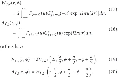
It is easy to see that the GFC includes as particular cases almost all definitions of the fractional convolution and cor-relation operations proposed before [57,58,59,60,61,62, 63,64,65,66,67,68,69,70]. Also the expressions for the cross-WD and cross-AF can easily be given in terms of the GFC; for the cross-WD and cross-AF expressed in polar co-ordinates [34],
Wf,g(r,φ)
=2 ∞
−∞Fφ+π/2(u)G ∗
φ+π/2(−u) exp
i2πu(2r)du, (17)
Af,g(r,φ)
= ∞
−∞Fφ+π/2(u)G ∗
φ+π/2(u) exp(i2πur)du,
(18)
we thus have
Wf,g(r,φ)=2Hf,g∗
2r,π 2,φ+
π
2,−φ+
π
2
, (19)
Af,g(r,φ)=Hf,g∗
r,π 2,φ+
π
2,−φ−
π
2
, (20)
respectively. The GFC system is represented schematically in Figure 2, indicating a general procedure to obtain the GFC.
In view of the canonical integral transform, a further gen-eralization of the convolution operationHf,g(x,M1,M2,M3) can be proposed as [69]
RM1H
f,g
x,M1,M2,M3
=RM2f(x) RM3g(x) ,
i
fg
Rβ
Rγ
× R−α Hf ,g
Figure 2: Schematic representation of the generalized fractional convolution system.
where the kernels of the three canonical integral transforms are parameterized by a matrix M(see (6)). This definition corresponds to the nonconventional convolution that is used in real optical systems under the paraxial approximation of the scalar diffraction theory, where the image and filter planes are shifted from their conventional positions [68,71]. As particular cases, the GFC and the Fresnel convolution can thus be realized. The introduction of the canonical convolu-tion operaconvolu-tion permits to find features similar to the ones of the fractional Fourier correlators and the Fresnel correlator, proposed several years ago in [71], and to treat easily the frac-tional correlator based on the modified fracfrac-tional FT [68].
Note that the GFC of a one-dimensional signal is a func-tion of four variables:x,α,β, andγ. The angle variables are often considered as parameters, and the function becomes one-dimensional. As we will see below in Sections5and6, optical signal processing allows to treat the GFC as a two-dimensional function, where one of the parameters is con-sidered as the second coordinate. The choice of the parame-ters and the number of variables of the GFC depends on the particular application. In Sections5–8, we will consider the applications of the GFC for phase retrieval, signal character-ization, pattern recognition, and filtering tasks, respectively.
5. FRACTIONAL POWER SPECTRA FOR PHASE RETRIEVAL
Phase retrieval from intensity information is an important problem in many areas of science, including optics, quantum mechanics, X-ray radiation, and so forth. In particular, non-interferometric techniques have attracted considerable atten-tion recently. In this secatten-tion, we consider the applicaatten-tion of fractional FT systems for the phase retrieval problem.
The squared moduli of the fractional FT, also called frac-tional power spectra, correspond to the projection of the WD upon the direction at an angleαin phase space. Note also that the fractional power spectrum is the particular case of the GFC
Fα(u)2
=Hf,f∗(u, 0,α,−α). (22)
Fractional power spectra play an important role in frac-tional optics: they are related to the intensity distributions at the output plane of a fractional FT system and therefore can be easily measured in optics. The set of fractional power spectra forα∈[0,π] is called the Radon-Wigner transform [116], because it defines the Radon transform of the WD. The WD can be obtained from the Radon-Wigner transform by
applying the inverse Radon transform [101, Chapter 8]. This is a basis for phase-space tomography [32], a method for ex-perimental determination of the complex field amplitude in the coherent case or the two-point correlation function for partially coherent fields, from the measurements of only in-tensity distributions. Application of cylindrical lenses allows the reconstruction of two-dimensional optical fields.
In the case of coherent optical signals, other methods for phase retrieval based on the measurements of fractional power spectra have been proposed. One of them is related to the estimation of the instantaneous spatial frequencyΞ(x) from two close fractional power spectra. It was shown that the instantaneous frequency is related to the convolution of the angular derivative of the fractional power spectrum and the signum function [33],
ΞFβ(x)=
∞
−∞ξWf(xcosβ−ξsinβ,xsinβ+ξcosβ)dξ ∞
−∞Wf(xcosβ−ξsinβ,xsinβ+ξcosβ)dξ
= 1
2Fβ(x)2 ∞
−∞
∂Fα
x2 ∂α
α=β
sgnx−xdx,
(23)
where sgn(x)= ±1 forx≷0. Moreover, since the instanta-neous frequency is the phase derivative of the fractional FT of a signal,
2πΞFβ(x)= dϕβ(x)
dx , (24)
where ϕβ(x) = argFβ(x), the complex field amplitude up to a constant phase factor can be reconstructed from only two close fractional power spectra [33,34,35]. This method has been demonstrated on different examples of multicom-ponent and noisy signals and exhibits high quality of phase reconstruction [35]. Note that a similar method of phase re-trieval can be applied for any one-parameter canonical trans-form [36]. Thus, in the case of the Fresnel transform, we can mention a noniterative approach for phase retrieval in free space, based on the so-called transport-of-intensity equation in optics, proposed by Teague [37] and then further devel-oped by others.
In the case that two fractional power spectra are known for angles which are not close to each other, iterative methods of phase retrieval can be applied [38,39,40]. These methods are a generalization of the iterative Gerchberg-Saxton algo-rithm, designed for the recovery of a complex signal from its intensity distribution and power spectrum.
Another method for phase retrieval is based on a sig-nal decomposition as a series of orthogosig-nal Hermite-Gauss modes [41]. It has been shown that if a coherent optical sig-nal contains only a finite number of Hermite-Gauss modes
N, then it can be reconstructed from the knowledge of its 2N
A further method for phase retrieval is based on filter-ing of the optical field in fractional Fourier domains [42]. Indeed, the phase derivativedϕ/dx, and therefore the phase
ϕ(x) up to a constant term, can be reconstructed from the knowledge of the intensity|f(x)|2 and the intensity distri-butions at the output of two fractional FT filters with mask
u:
dϕ(x)
dx =π
R−αFα(u)u(x)2−RαF
−α(u)u(x)2
xf(x)2sin 2α .
(25)
The efficiency of this approach has been demonstrated by nu-merical simulations. A simple optical configuration for the experimental realization of the method was discussed in [42].
6. FRACTIONAL POWER SPECTRA FOR OPTICAL BEAM CHARACTERIZATION
Since the AF, the WD, and other bilinear distributions of two-dimensional optical signals are functions of four variables, their direct application for the analysis and characterization is limited. Mostly the moments of these distributions are used for beam characterization. The normalized moments
µpqrsof the WD are defined by
µpqrsE= ∞
−∞ ∞
−∞ ∞
−∞ ∞
−∞W(x,ξ;y,η)
×xpξqyrηsdx dξ d y dη (p,q,r,s≥0), (26)
where the normalization is with respect to the total energyE
of the signal (and henceµ0000=1). Note that in a first-order optical system, with a symplectic ray transformation matrix, the total energyEis invariant. The low-order moments rep-resent the global features of the optical signal such as total energy, width, principal axes, and so forth. Thus the second-order moments of the WD (p+q+r+s =2) are used as a basis of an International Organization for Standardization standard of beam quality. The combination of the second-order moments (µ1001−µ0110)E, for instance, describes the orbital angular momentum of the optical beam, which is ac-tively used for the description of vortex beams [117]. The moments of higher order are related to finer details of the optical signal.
Note that forq = s = 0 and for p = r = 0, we have the position and frequency moments, which can easily be ob-tained from measurements of the intensities in the signal and the Fourier domain, respectively:
µp0r0E= ∞
−∞ ∞
−∞x pyrF
0(x,y)2dx d y, (27)
µ0q0sE= ∞
−∞ ∞
−∞ξ qηsF
π/2(ξ,η)2dξ dη. (28)
Since in optics only intensity distributions can be measured directly, it was proposed in [43] to apply fractional FT sys-tems in order to calculate other moments from the intensity
moments. It was shown that the moments at the output plane of a separable fractional FT system, with fractional anglesα
andβin thex- and the y-direction, respectively, are related to the input ones as
µout pqrs=
p
k=0 q
l=0 r
m=0 s
n=0
p k
q l
r m
s n
×(−1)l+n(cosα)p−k+q−l(sinα)k+l(cosβ)r−m+s−n ×(sinβ)m+nµinp−k+l,q−l+k,r−m+n,s−n+m,
(29)
and for the intensity moments in particular, we have
µoutp0r0= p
k=0 r
m=0
p k
r m
(cosα)p−k(sinα)k
×(cosβ)r−m(sinβ)mµin
p−k,k,r−m,m.
(30)
From (30) a set of fractional FT systems can be found for which the input moments can be derived from knowledge of the intensity moments in the output, that is, from fractional power spectra for selected angles αand β. It was demon-strated [43] that in order to find allnth order moments—and we have (n+ 1)(n+ 2)(n+ 3)/6 of such moments—we need
Nfractional power spectra, whereN=(n+ 2)2/4 for evenn andN =(n+ 1)(n+ 3)/4 for oddn. Moreover,N−(n+ 1) spectra have to be anamorphic, that is, spectra with nonequal fractional order for the two transversal coordinates (α=β). In particular, we need 2 fractional spectra to find the 4 first-order moments, 4 fractional spectra (one of which has to be anamorphic) to find the 10 second-order moments, 6 frac-tional spectra (with 2 anamorphic ones) to find the 20 third-order moments, and so forth.
Regarding the evolution of the second-order moments in a fractional FT system, we can find the fractional domain where the signal has the best concentration or where it is the most widely spread, by calculating the zeros of the angular derivatives of the central momentsµp0r0(α,β). This analysis [33,34] is helpful, for example, in search for an appropri-ate fractional domain to perform filtering operations [45]. Smoothing interferograms in the optimal fractional domain leads to a weighted WD with significantly reduced interfer-ence terms of multicomponent signals, while the auto terms remain almost the same as in the WD. In general, based on this approach, optimal signal-adaptive distributions can be constructed with low cost [46].
The way to determine the moments from measurements of intensity distributions as described by (30) has been gen-eralized to the case of arbitrary separable first-order optical systems [44]. Using an equation similar to (29), one can eas-ily determine the evolution of these moments during propa-gation of the beam in any first-order optical system; in partic-ular, this was applied to the analysis of optical vortices [47].
It was shown [50,51,52,53,54,55,56] that the frac-tional FT spectra as well as the Fresnel spectra are also useful for the analysis of fractal signals. Thus the hierarchical struc-ture of the fractal fields and its main characteristics such as fractal dimension, Hurst exponent, scaling parameters, frac-tal level, and so forth, can be obtained from the analysis of the fractional spectra for the angular region from 0 toπ/2 [50,51,52,53]. Since in this region the fractional FT spec-tra and the Fresnel spec-transform specspec-tra differ only by a scal-ing parameter, the Fresnel diffraction is applied for this task [51,52,55]. Recently the experimental fractal tree of triadic Cantor bars has been constructed from the observation of the evolution of diffraction patterns in free space [54]. The gen-eral properties of the Fresnel diffraction by structures con-structed through the multiplicative iterative procedure have been studied in [56].
7. GENERALIZED FRACTIONAL CONVOLUTION FOR PATTERN RECOGNITION
A great part of the proposed applications of the GFC is re-lated to pattern recognition tasks [57,60,66,67,68,69,70, 71,72,73,74]. It was shown [66,67] that for this purpose, the following relation between the angular parameters has to hold:
cotα=cotβ+ cotγ. (31)
Then the amplitude of the GFC is expressed in the form [66] Hf,g∗(x,α,β,γ)
=C
∞
−∞f
sinβ
sinγ
xsinγ
sinα−y
g∗y
×exp
iπ y2cotα
1 + cotγcotβ
1 + cot2β
−iπ yx sin 2β
sinαsinγ
d y,
(32)
where C is a constant for fixedα,β, and γ. The quadratic phase factor under the integral vanishes—which brings the integral in the form of a windowed FT—if cotα(1 + cotγcotβ) =0. In the case cotα =0 (and henceα = π/2 andγ= −β) which is usually considered,Hf,g∗(r,π/2,β,−β) corresponds to radial slicesAf,g(r,β−π/2) of the cross-AF of the signals f(x) andg(x) (cf. (20)).
If the position and the size of the object is known, then the correlation operationHf,g∗(x,α,β,−β) for pattern recog-nition can be performed in any fractional domainβ, since the auto-AF has a maximum at the coordinate originr =0. Nevertheless, in spite of the fact that the magnitude of the correlation maximum is the same in any fractional domain, the forms of the correlation peaks are different. It was shown [70] on the example of a rectangular function that the nar-rowest correlation peak is observed in the fractional domain with fractional angleβ=0. Note also that the object is usu-ally corrupted by noise, or is blurred. The characteristics of
ξ
β−π/2 u s
Figure3: Schematic representation of the cross-AF of two signals, before (solid line) and after (dashed line) shifting of one of the sig-nals.
the noise (except for white noise) in different fractional do-mains depend on the fractional angle [75]. The fractional correlation offers the flexibility to choose the domain where the effect of noise on the correlation operation is minimized. Moreover, for the recognition of complex or highly degraded objects, several fractional correlation operations for different angles can be performed in order to make the right decision. On the other hand, if the position of the object is un-known, the choice of the fractional domain is related to the tolerance to a shift variance of the correlation operation. A shift of the signal leads to a shift and a modulation of the cross-AF:
Af(y−s),g(y)(x,ξ)=Af(y),g(y)(x−s,ξ) exp(−iπsξ). (33)
Then the form of the AF radial slices of a shifted signal is changing except for the angle corresponding to the ordinary correlation (seeFigure 3).
Therefore fractional correlations are shift variant forβ=
π/2 +nπ. Thus if in the conventional correlator a shift of the object results in a shift with opposite sign of the cor-relation peak at the output plane, the shape of the peak is also changed in the fractional correlator. This effect increases with decreasing parameterβfromπ/2 down to 0. For largeβ, the fractional correlator is almost shift invariant, whereas for smallβ, it becomes strongly shift variant. Note that there are applications, such as cryptography or image coding, where the location of the object can be as important as its form. In these cases fractional correlators with fractional parameterβ, 0< β < π/2, must be used.
The shift tolerance condition is usually written in the form [29,59,60]πsσcotβ 1, wheresis the signal shift andσthe signal width. More precisely, the shift variance de-pends on the fractional order, the signal size, and also the form of the AF.
orthogonal coordinates and thus to better control the shift variance. In order to recognize a letter on a certain line of the text, for example, one can choose the parameter βx =
π/2 andβy < π/2 while the filter corresponds to the inverse fractional FT with parametersβx,βyof a letter situated on a given line. The exciting results demonstrating the efficiency of shift-variant pattern recognition in the fractional domain can be found in [72,73,74].
The fractional correlation operation can be performed in optics by a fractional Van der Lugt correlator [72,73,74] or by a nonconventional joint-transform correlator [118].
In order to maximize the Horner efficiency of the correla-tion operacorrela-tion, phase-only filters are often used. It was shown in [76] that in general, the phase of the fractional FT for
α =nπ contains more information about the signal/image than the amplitude. Therefore the phase-only filters can also be applied in the fractional Fourier domain. The develop-ment of liquid crystal spatial light modulators allows their relatively simple implementation in optics.
Another particular case of GFC which can be applied for recognition tasks is related to the fractional FT of the or-dinary correlation operation [23]Hf,g∗(x,α,π/2,−π/2). We believe that this type of operation can be useful for anglesα
at the region nearπ/2 in order to improve the performance of the conventional correlation operation. Thus it was shown [77] that forαslightly different fromπ/2, the performance of the joint-transform correlator improves and higher correla-tion peaks are observed. Efficient use of the light source and a larger joint-transform spectrum were achieved. Moreover, for these anglesα, the correlator still remains shift invariant. Nevertheless using anglesαfar fromπ/2 leads to confusing results for interpreting the correlation peaks. Indeed, if the conventional correlation operation does not produce a clear local maximum and is almost constant, then a sharp peak in fractional correlationHf,g∗(x,α≈0,π/2,−π/2) can appear.
8. GENERALIZED FRACTIONAL CONVOLUTION FOR FILTERING AND DATA PROTECTION
We consider now the filtering operation in the fractional do-main. The parameters of the GFC in this case depend on the particular application of filtering. If the filter is used for im-provement of image quality or for manipulation of the image
f in order to extract its features (e.g., for edge detection or image deblurring), then we have to chooseβ=αin order to represent the result of filtering in the position domain. Since we are free to assign an arbitrary fractional domain for the filter functiong, we can as well putγ=α. Thus the complete operation leads to theHf,g(x,α,α,α). The useful properties of this type of GFC,
RβH
f,g(x,α,α,α)
(u)=HFβ,Gβ(u,α−β,α−β,α−β),
Hf,g(x,α,α,α)=Hf,g(x,α+π,α+π,α+π), (34)
were proved in [62]. Moreover, this type of convolution op-eration is associative for a fixed parameterα.
The GFCHf,g(x,α,α,α) has been found very powerful for noise reduction, if the noise is separable from the signal or very well concentrated in some fractional domain [57]. It was shown that in particular for chirp-like noise, the per-formance of filtering in a fractional domain is more relevant [24, 29]. Since the fractional FT of a chirp becomes pro-portional to a Dirac-delta function in an appropriate frac-tional domain, it can be detected as a local maximum on the Radon-Wigner transform map and then easily removed by a notch filter, which minimizes the signal information loss.
Several applications of fractional FT filtering systems for industrial devices have been proposed recently.
Chirp detection, localization, and estimation via the frac-tional FT formalism are applied now in different areas of science. Appropriate filtering in fractional domains, which allows to extract linear chirps out of a multicomponent and noisy signal, is used to analyze the propagation of acoustic waves in a dispersive medium [119]. In particular, the non-linear effects due to the Helmholtz resonators are considered. A new spatial filtering technique for partially coherent light in the fractional Fourier domain [120] was proposed to improve image contrast and depth of focus in projection photolithography. Unlike the currently applied pupil method of filtering in the Fourier domain, the fractional filter can be placed at any location along the projection optical path other than the pupil plane. On the examples of designed phase fil-ters for contact hole and line-space patterns, it was demon-strated that the fractional FT filtering technique can signif-icantly improve image fidelity, reduce the optical proximity effect, and increase the depth of focus.
Optical technologies play an increasing role in securing information [121]. Also the GFC found its way into security protection: encryption and watermarking techniques origi-nally proposed for the Fourier domain were generalized to the fractional domain.
Optical image encryption by random-phase filtering in the fractional Fourier domain was proposed in [78,79]. It can be described by the GFCHf,g(x,α,β,β), where the phase mask Gβ and the parameters α and β are the encryption codes. This procedure was further generalized by application of the cascaded fractional FT with random-phase filtering [80]. In order to encode the image, the fractional transform is performed and random-phase is introduced by means of a spatial light modulator. After repeating this procedure sev-eral times, the encrypted image is obtained. In order to de-code it, not only the information about the used random-phase masks has to be known, but also the parameters and the types of the fractional transforms. It was demonstrated that it is impossible to reconstruct the image using the cor-rect masks but with the wrong fractional orders. Without increasing the complexity of the hardware, the fractional-Fourier optical image encryption system has additional keys provided by the fractional order of the fractional convolution operation. Due to the double domain properties of the frac-tional FT, the algorithm demonstrates the robustness to the blind deconvolution.
Thus in [81] the combination of a jigsaw transform and a lo-calized fractional FT was applied. The image to be encrypted is divided into independent nonoverlapping segments, and each segment is encrypted using different fractional param-eters and two statistically independent random-phase codes. The random-phase codes, the set of fractional orders, and the jigsaw transform index are the keys to the encrypted data. The encryption by juxtaposition of sections of the image in fractional Fourier domains without random-phase screen keys was proposed in [82].
Another encryption technique discussed in [83] is based on a method of phase retrieval using the fractional FT. The encrypted image consists of two intensity distributions, ob-tained in the output of two fractional FT systems of different fractional orders, where the input of each system is formed by the 2D complex signal multiplied by a random-phase mask. The two statistically independent random-phase masks and the fractional orders form the encryption key. Decryption is based on the correlation property of the fractional FT, which allows to recover the signal recursively.
The implementation of a fully phase encryption system, using a fractional FT to encrypt and decrypt a 2D phase im-age obtained from an amplitude imim-age, was reported in [85]. A comparative analysis of the encryption techniques based on the implementation of the fractional FT has been done in [84].
Watermarking is another widely applied data protec-tion operaprotec-tion. A watermarking technique in the fracprotec-tional domain was proposed in [86, 87]. In this case, the GFC
Hf,g(x,α,α,α) is commonly used. In order to include the wa-termark, theα-fractional FT of the image is performed. The signature has to be a function that is spread in the image do-main and well localized in the fractional dodo-mainα. Usually a chirp signal, which becomes aδ-function in a certain frac-tional domain and should be spread in the image domain, is used. Introducing the watermark and performing the inverse fractional FT, finally we obtain the protected image. Usually several watermarks in different fractional FT domains are in-troduced. Only the owner of the image who knows the all fractional domains will be able to remove them. This water-marking technique is robust to translation, rotation, crop-ping, and filtering [86,87].
9. GENERAL ALGORITHM FOR THE
FRACTIONALIZATION OF CYCLIC TRANSFORMS We have considered the properties and application of the fractional FT. Now the following key questions arise.
(i) Is this fractional FT unique? Or is it possible to gener-ate other fractional FTs?
(ii) How can we generate the fractional version of other transformations, for example, Hilbert, sine, cosine?
(iii) Do fractional transforms have some common prop-erties?
In order to answer these questions, we will consider the procedure of fractionalization of a given transform [27,28]. Similar approaches for fractionalization of the integral trans-form, and the FT in particular, were reported in [122] and
[123], respectively. We will restrict ourselves to the consider-ation of cyclic transforms. There is a long list of linear trans-forms, actively used in optics and signal/image processing, which belong to this class of cyclic transforms. Thus, ifRis an operator of a linear integral transform, see (1), this trans-form is a cyclic one, if it produces the identity transtrans-form when it acts an integer number of timesN:
RNf(x)(u)= f(u). (35)
For example, the Fourier and Hilbert transforms are cyclic with a periodN=4, and the Hankel and Hartley transforms have a periodN =2. Cyclic canonical transforms of period
Nwith kernelK(x,u)=KM(x,u) (cf. (4)),
K(x,u)=√1
ibexp
iπax
2+du2−2ux
b
, (36)
wherea+d=2 cos(2πm/N) andmandNare integers, were mentioned in [124].
All cyclic transforms have some common properties. In particular, the eigenvalues of cyclic transforms can be rep-resented as A = exp(i2πL/N), where L is an integer. In-deed, let Φ(x) be an eigenfunction of R with eigenvalue
A= |A|exp(iϕ); from (35) one gets thatAN =1, and hence |A| =1 andϕ=2πL/N.
InSection 2, we have formulated the requirements for the fractionalR-transformRp, where pis the parameter of the fractionalization: continuity ofRpfor any real valuep; addi-tivity ofRpwith respect to the parameterp; reproducibility of the ordinary transform for integer values of p:R1 =R andR0 =I. In the case of cyclic transforms, we obviously demand thatRN =I.
Let us analyze the structure of the kernelK(p,x,u) of a fractionalR-transform with periodN. Due to its periodicity with respect to the parameterp, one can representK(p,x,u) in the form
K(p,x,u)= ∞
n=−∞
kn(x,u) exp i
2π pn N
, (37)
where the coefficientskn(x,u) have to satisfy the system ofN
equations [27]
K(l,x,u)= ∞
n=−∞
kn(x,u) exp
i2πln N
(38)
withl =0,. . .,N−1. From the additivity property for the fractional transform, it follows that the coefficients have to be orthonormal to each other [27,28]:
∞
−∞kn(x,u)km(u,y)du=δn,mkn(x,y), (39)
Note that all coefficientskn+mN(x,u) for fixednand an arbitrary integermhave the same exponent factor in the sys-tem of (38). Therefore, we can rewrite (38) as
K(l,x,u)= N−1
n=0 exp
i2πln N
∞
m=−∞
kn+mN(x,u). (40)
If we introduce the new variablesCn(x,u), which are the par-tial sums of the coefficients in the Fourier expansions (37) and (38),
Cn(x,u)= ∞
m=−∞
kn+mN(x,u), (41)
equation (40) reduces to a system ofNlinear equations with
Nvariables. This system has a unique solution [27]
Cn(x,u)= 1
N
N−1
l=0 exp
−i2πln
N
K(l,x,u). (42)
It is easy to see that the variablesCnsatisfy a condition similar to (39):
∞
−∞Cn(x,u)Cm(u,y)du=δn,mCn(x,y). (43)
Note that some partial sums for certain transforms may be equal to zero. As we will see further on, this is the case for the Hilbert transform, for instance.
So, if we find the coefficientskn(x,u) that satisfy the con-dition (39) and whose partial sums are given by (42), we can construct the fractional transform. In general, there are a number of sets{kn(x,u)}that generate fractional transforms of a givenR-transform.
10. N-PERIODIC FRACTIONAL TRANSFORM KERNELS WITHNHARMONICS
We first construct the fractional transform kernel with N
harmonics, where N is the period of the cyclic transform. Then every sumCn(x,u) (n∈[0,N−1]) contains only one elementkn+ϕn(x,u)=Cn(x,u) from the decomposition (37),
where ϕn = mN andmis an arbitrary integer. Therefore, in the general case, the kernel of the fractionalR-transform withNharmonics can be written as
K(p,x,u)= N−1
n=0
kn+ϕn(x,u) exp
i2π pn+ϕn
N
= 1
N
N−1
l=0
K(l,x,u) N−1
n=0 exp
−i2πln
N
×exp
i2π pn+ϕn
N
.
(44)
This equation provides a formula for recovering the con-tinuous periodic function K(p,x,u) from its N samples
K(l,x,u), under the assumption that the spectrum of
K(p,x,u) contains only N harmonics at the frequencies {ϕ0, 1 +ϕ1,. . .,n+ϕn,. . .,N−1 +ϕN−1}.
If we putϕn = 0 (n = 0, 1,. . .,N−1), we obtain the fractional transform with the kernel
K(p,x,u)= 1
N
N−1
l=0 exp
iπ(N−1)(p−l)
N
× sin
π(p−l)
sinπ(p−l)/NK(l,x,u)
(45)
proposed by Shih in [125]. In particular, this formula is used as the definition of a kind of fractional FT (for the continu-ous as well as the discrete case) [125,126].
WithNan odd integer and choosingNnonzero coeffi -cients in the decomposition (37) with indicesj= −(N−1)/
2,. . ., 0,. . ., (N−1)/2 (corresponding to the indicesn+mN
form = 0 andn = 0, 1,. . ., (N−1)/2, and m = −1 and
n=(N−1)/2 + 1,. . .,N−1), we obtain the kernel
K(p,x,u)= 1
N
N−1
l=0
sinπ(p−l)
sinπ(p−l/N]K(l,x,u). (46)
This equation corresponds to the recovering procedure of a band-limited periodic function from its values on equidis-tant sampling points [127]. In particular, ifK(l,x,u) is real for integerl=0, 1,. . .,N−1, then the kernel of the fractional transform determined by (46) is real, too. It also means that the Fourier spectrum ofK(p,x,u) with respect to the param-eterpis symmetric:|kj| = |k−j|.
As an example, we consider the general expression (44) for the kernel of the fractional R-transform with period 4 (which is the case for the Fourier and Hilbert transforms):
K(p,x,u)=1 4
3
l=0
K(l,x,u)S(l) (47)
withS(l)=!3
n=0exp(−inlπ/2) exp[i(n+ϕn)pπ/2].
Note that for the Hilbert transform, the number of har-monics reduces to two, because C0(x,u) = C2(x,u) = 0, which follows fromK(0,x,u)= −K(2,x,u) andK(1,x,u)= −K(3,x,u). From (44) we then conclude that the fractional Hilbert transform kernel can be written as
K(p,x,u)=expi(m1+m3+ 1)pπ
× "
K(0,x,u) cos
m3−m1+1 2
pπ
−K(1,x,u) sin
m3−m1+1 2
pπ
# ,
wherem1andm3are integers. In particular, for the casem1=
m3=0 (kn=0 ifn=1, 3), one gets
K(p,x,u)=exp(ipπ)
×
K(0,x,u) cos
pπ
2
−K(1,x,u) sin
pπ
2
,
(49)
while for the casem1=0 andm3= −1 (kn=0 ifn= −1, 1), the common form for the fractional Hilbert transform [94] with a real kernel is obtained:
K(p,x,u)=K(0,x,u) cos pπ
2
+K(1,x,u) sin pπ
2
.
(50)
Therefore, even for the same number of harmonics, there are several ways for the fractionalization of cyclic transforms.
11. FRACTIONAL TRANSFORM KERNELS CONSTRUCTION USING EIGENFUNCTIONS OF CYCLIC TRANSFORMS
In the case that the set of orthonormal eigenfunctions of the cyclic transform exists, one can construct fractional kernels with a number of harmonicsM > N, whereNis the period of the cyclic transform [27,28].
Suppose that there is a complete set of orthonormal eigenfunctions {Φn} of the operator R with eigenvalues {An = exp(i2πLn/N)},n = 0, 1,. . .(see Section 9). Then we can represent a kernel of theR-transform of the integer powerqas
K(q,x,u)= ∞
n=0
Φn(x)AqnΦ∗n(u)
= ∞
n=0
Φn(x) exp i2πqL
n
N
Φ∗ n(u).
(51)
One of the possible series of kernels for the fractional R-transform can then be written in the form
K(p,x,u)= ∞
n=0
Φn(x) exp
i2π
Ln
N +ln
p
Φ∗
n(u), (52)
wherelnis an integer and indicates the location of the har-monics. This kernel satisfies the additivity condition due to the orthonormality of the eigenfunctionsΦn(x).
Note that not all cyclic operators have a complete set of orthonormal eigenfunctions, as it is the case, for example, for the Hilbert operator, whose eigenfunctionsΦ(x) are self-orthogonal. Nevertheless, the majority of cyclic transforms of interest in optics, such as Fourier, Hartley, Hankel, and so forth, have this set. For the Fourier and Hartley transforms,
Φn(x) are the Hermite-Gauss modes [15,16]
Φn(x)=21/42nn!−1/2H n
x√2πexp−πx2, (53)
where Hn(x) are the Hermite polynomials; for the Han-kel transform of different orders,Φn(x) are the normalized Laguerre-Gauss functions [128,129].
The canonical fractional FT kernel, discussed in the pre-vious sections, can be obtained from (52) as a particular case:
Ln= −nandln=0,
KF(p,x,u)
= ∞
n=0
Φn(x) exp
−inpπ 2
Φ∗ n(u)
=exp( inpπ/4)
isin(pπ/2)exp
iπ
x2+u2cos(pπ/2)−2ux sin(pπ/2)
(54)
(cf. (11)). The fractional Hankel transform, defined by (52) forLn = −nandln = 0 andΦn(x) being the normalized Laguerre-Gauss functions, describes the propagation of ro-tationally symmetric optical beams through a medium with a quadratic refractive index [128,129]. The kernels of these transforms contain an infinite number of harmonics.
We rewrite (52) in the form
K(p,x,u)= ∞
n=−∞
zn(x,u) exp
i2πnp N
. (55)
Here zn(x,u) is a sum of the elementsΦj(x)Φ∗j(u) over j, where Φj(x) is the eigenfunction of theR-transform with eigenvalue exp(i2πn/N). Thus for the case of the canonical fractional FT,
KF(p,x,u)= ∞
n=0
Φn(x) exp
−inpπ 2
Φ∗ n(u)
= 0
n=−∞
zn(x,u) exp
inpπ
2
,
(56)
the coefficientszn(x,u) vanish for positivenandzn(x,u)=
Φn(x)Φ∗n(u) forn ≤0. As we will see below, the fractional Hartley transform [27] can be represented in the form
K(p,x,u)= ∞
n=0
exp(−iπnp)z−n(x,u),
z−n(x,u)=Φ2n(x)Φ2n(u) +Φ2n+1(x)Φ2n+1(u). (57)
It is easy to see from (55) that we can generate another kernel series withMharmonics,
K(p,x,u)= M−1
n=0 exp
i2πnp M
∞
m=−∞
zn+mM(x,u), (58)
which satisfy the requirements for the fractional transforms. Here the sums of the elementszj(x,u),
kn(M,x,u)= ∞
m=−∞