DOI: 10.1534/genetics.108.093690
A Computational Approach to the Functional Clustering of Periodic
Gene-Expression Profiles
Bong-Rae Kim,*
,1Li Zhang,
†,1Arthur Berg,* Jianqing Fan
‡and Rongling Wu*
,2*Department of Statistics, University of Florida, Gainesville, Florida 32611,†Department of Quantitative Health Sciences, Cleveland
Clinic Foundation, Cleveland, Ohio 44195 and‡Department of Operation Research and Financial Engineering,
Princeton University, Princeton, New Jersey 08544
Manuscript received July 7, 2008 Accepted for publication August 5, 2008
ABSTRACT
DNA microarray analysis has emerged as a leading technology to enhance our understanding of gene regulation and function in cellular mechanism controls on a genomic scale. This technology has advanced to unravel the genetic machinery of biological rhythms by collecting massive gene-expression data in a time course. Here, we present a statistical model for clustering periodic patterns of gene expression in terms of different transcriptional profiles. The model incorporates biologically meaningful Fourier series approximations of gene periodic expression into a mixture-model-based likelihood function, thus producing results that are likely to be closer to biological relevance, as compared to those from existing models. Also because the structures of the time-dependent means and covariance matrix are modeled, the new approach displays increased statistical power and precision of parameter estimation. The approach was used to reanalyze a real example with 800 periodically expressed transcriptional genes in yeast, leading to the identification of 13 distinct patterns of gene-expression cycles. The model proposed can be useful for characterizing the complex biological effects of gene expression and generate testable hypotheses about the workings of developmental systems in a more precise quantitative way.
A
LMOST all of life’s phenomena populating the earth can be described in terms of periodic rhythms that result from the planet’s rotation and orbit around the sun (Goldbeter 2002). Cell division (Mitchison 2003), circadian rhythms (Crosthwaite 2004; Prolo et al. 2005), morphogenesis of periodic structures such as somites in vertebrates (Dale et al. 2003), and the complex life cycles of some micro-organisms (Lakin-Thomasand Brody 2004; Rovery et al.2005) are all excellent representatives of biological rhythms. From a mechanistic perspective, rhythmic behavior arises in genetic and metabolic networks as a result of nonlinearities associated with various modes of cellular regulation.The complexity and inherent periodicity of rhythmic processes can be well described by mathematical mod-els. For example, mathematical models of increasing complexity for the genetic regulatory network produc-ing circadian rhythms in the fly Drosophila predict the occurrence of sustained circadian oscillations of the limit cycle type (Leloupet al.1999). When incorporat-ing the effect of light, the models account for phase shifting of the rhythm by light pulses and for entrain-ment by light–dark cycles. The models also provide an
explanation for the long-term suppression of circadian rhythms by a single pulse of light. Stochastic simulations were developed to test the robustness of circadian oscillations with respect to molecular noise (Gonze et al.2002, 2003).
The recent development of gene-expression technol-ogies has offered biologists a unique opportunity to more closely study the mechanisms that control a particular biological rhythm. Panda et al. (2002) em-ployed high-density oligonucleotide arrays to trace gene expression in mouse tissue samples taken every 4 hr during two complete circadian cycles. They also identi-fied clusters of circadian-regulated genes among.7000 genes with a cosine wave-fitting algorithm (Harmer et al.2000). About 650 cycling transcripts were detected to be under circadian regulation specific to either the suprachiasmatic nuclei or the liver. These studies allowed the authors to understand how the major oscillator in the suprachiasmatic nuclei and the liver regulates behavioral and physiological rhythms in the whole organism.
To associate the profile of gene expression with a physiological function of interest, it is crucial to cluster the types of gene expression on the basis of their periodic patterns. Statistical modeling and algorithms play a central role in cataloging dynamic gene-expres-sion profiles. While various computational models have been developed for gene clustering based on 1These authors contributed equally to this work.
2Corresponding author:Department of Statistics, University of Florida, Gainesville, FL 32611. E-mail: rwu@stat.ufl.edu
static microarray data (Eisen et al. 1998; Ghosh and Chinnaiyan2002; McLachlanet al.2002; Ramoniet al. 2002; Fan and Ren2006), considerable attention has been paid to methodological derivations for detecting temporal patterns of gene expression in a time course based on functional principal component analysis or mixture model analysis (Holteret al.2001; Qianet al. 2001; Bar-Josephet al.2003; Luanand Li2003; Park et al. 2003; Wakefield et al. 2003; Ernst et al. 2005; Storeyet al.2005; Maet al.2006; Nget al.2006; Inoue et al.2007). In particular, Luanand Li(2004) proposed a statistical model for characterizing different types of periodic rhythms of gene expression. These methods show some unique utilization to identify genes with varying expression profiles over time, providing new tools to elucidate a comprehensive picture of the life process.
A common feature of these clustering methods is that they model time-dependent gene-expression profiles using nonparametric approaches, such as cubic splines. Although nonparametric approaches are statistically flexible and computationally fast, they often do not provide rigorous biological interpretations of results even if the gene-expression data analyzed contain some biologically meaningful patterns. This article was moti-vated by the fundamental idea that key features of many biological processes can be described by parsimonious mathematical equations. For example, Frank (1926) used the Fourier series to approximate periodic and quasi-periodic biological phenomena. Attingeret al. (1966) provided a detailed mathematical formulation of this approximation for a biological rhythmic system through both theoretical and experimental approa-ches. Fourier series approximation as an analytical tool (Priestley1981) has been widely applied to study the mechanisms and patterns of biological rhythmicity, including the cyclic organization of preterm and term neonates during the neonatal period (Begum et al. 2006) and pharmacodynamics (Magerand Abernethy 2007).
Fourier approximation has also been used to model periodic gene expression, leading to the detection of periodic signals in various organisms including yeast and human cells (Spellmanet al.1998; Wichertet al. 2004; Kimet al.2006). Glynnet al.(2006) proposed a Lomb–Scargle periodogram approach based on the fast Fourier transform to model unevenly spaced gene-expression time series and then characterize periodic patterns of gene expression by using a multi-ple-hypothesis testing procedure with a controlled false discovery rate. Our statistical model presented in this article integrates the Fourier series approximation into a mixture-model framework to mathematically cluster microarray genes on the basis of their distinct patterns of periodic expression. The advantage of this mixture-based model includes its solid statistical foundation of testing the number of gene clusters. Furthermore,
through the implementation of the Fourier series approximation, it is possible to test several biologically meaningful characteristics such as sharp peaks in the ordinary periodograms calculated from the Fourier transform of the time series (Durbin1967). We use a published example for cell cycle-regulated genes in
Saccharomyces cerevisiae(Spellmanet al.1998) to validate the new model. The statistical behavior of the model is examined through simulation studies.
METHODS
Mixture model:Finite mixture models (McLachlan and Peel 2000) have been widely used to model the distributions of a variety of random phenomena. Mul-tivariate normality is generally assumed for mulMul-tivariate data of a continuous nature. This multivariate normal mixture model is employed to detect different patterns in gene-expression profiles.
Assume thatngenes are measured at multiple time points. Our model is able to consider unevenly spaced time intervals and different measurement schedules for each gene. Let yi¼ ðyiðti1Þ;. . .;yiðtiTiÞÞ be the Ti
-dimensional gene-expression data for genei. Suppose there are J components in the mixture model. This means that any one of the genes (i) is assumed to arise from one (and only one) of the J possible periodic patterns of expression, the distribution of whose ex-pression data is expressed as theJ-component mixture probability density function;i.e.,
yi fiðyi;v;ui;SiÞ ¼ XJ
j¼1
vjfijðyi;uij;SiÞ; ð1Þ
wherev¼ ðv1;. . .;vJÞis the mixture proportions that are nonnegative and sum to unity; ui 5 (ui1,. . ., uiJ)
contains the component- (or pattern-) specific mean vector for genei; andSicontains residual variances and covariances among theTitime points for geneithat are common for all gene-expression patterns. The proba-bility density function of thejth gene-expression pattern or cluster, fijðyi;uij;SiÞ, is assumed to be multivariate normal with mean vectoruij¼ ðuijðti1Þ;. . .;uijðtiTiÞÞand
common covariance matrixSi.
From the above analysis, different gene-expression patterns can be detected by estimating the number of mixture components, the time-dependent means of each component, and the covariance matrix. By com-paring the differences of the mean vector among different components, it is possible to test how response curves differ among different components and, further, to address fundamentally important biological issues regarding the interplay between gene expression and biological rhythms.
approximation (Spellman et al. 1998). Fourier series approximations can assess periodicity, so we can identify the genes whose RNA levels varied periodically within the cell cycle and, further, find the associated ampli-tudes and phases of these cycles by estimating the mathematical parameters in the Fourier series approx-imation. A general form of the Fourier signal is given as
sKðtÞ ¼a01 X‘
k¼1
akcos 2pkt
T
1X
‘
k¼1
bksin 2pkt
T
;
ð2Þ
wherea0is the average value ofsK(t) and the otherak andbkcoefficients are the amplitude coefficients that determine the times at which the gene achieves peak and trough expression levels, respectively, andT is the period of the signal of gene expression.
In practice, the Fourier series of Equation 2 can be approximated by the firstK11 term. By analyzing the error of the Fourier series approximation, expressed as the difference between the signal and the (K11)-term series,
eKðtÞ ¼a01 X‘
k¼K11 akcos
2pkt T
1 X
‘
k¼K11 bksin
2pkt T
;
it is found that, when a third-order approximation is used (i.e.,K53), the unused terms (k54,. . .,‘) from the series together are only3% of the signal. Thus, the time-dependent expression value of a gene can be adequately modeled by a Fourier series approximation of the first three orders. Let Quj denote the vector
containing Fourier parameters of various orders for the genes with patternj, which is specified as
Quj ¼
ða0j;a1j;b1j;TjÞ for the first order;
ða0j;a1j;b1j;a2j;b2j;TjÞ for the second order;
ða0j;a1j;b1j;a2j;b2j;a3j;b3j;TjÞ for the third order: 8
< :
ð3Þ
The mean expression value of geneiwhen its pattern isj
at time pointtitcan be approximated by these Fourier
series parameters;i.e.,
uijðtitÞ ¼sKðQuj;titÞ:
Modeling the covariance structure: A number of approaches can be used to model the covariance structure of serial measurements. A commonly used approach for structuring the covariance is the first-order autoregressive [AR(1)] model (Davidianand Giltinan 1995; Verbekeand Molenberghs2000). One advantage of using the AR(1) model is that it provides a general expression for calculating the determinant and inverse of the matrix for any number of time points measured. But it assumes variance stationarity and correlation
stationar-ity;i.e., the residual variance at different time points is the same, expressed ass2, and the correlation between two
different time points for gene i,tit1 andtit2, decreases exponentially inrwith time lag, expressed as corr(yiðtit1Þ;
yiðtit2ÞÞ ¼r
jtit1tit2j.
To remove the heteroscedastic problem of the re-sidual variance, which violates a basic assumption of the simple AR(1) model, two approaches can be used. The first approach is to model the residual variance by a parametric function of time, as proposed by Pletcher and Geyer(1999). But this approach needs to imple-ment additional parameters for characterizing the time-dependent change of the variance. The second approach is to embed Carrolland Ruppert’s (1984) transform-both-sides (TBS) model into the growth-incorporated finite mixture model (Wuet al.2004), which does not need any more parameters. Both empirical analyses with real examples and computer simulations suggest that the TBS-based model can increase the precision of parame-ter estimation and computational efficiency. Further-more, the TBS model preserves original biological means of the curve parameters although statistical analyses are based on transformed data. In this study, we used the TBS-based AR(1) model, with the structuring parameters arrayed inQv.
Computational algorithm: The EM algorithm and Nelder–Mead simplex algorithm were used to estimate the unknown parameters V¼ ðfvj;Qujg
J
j¼1;QvÞ. The observed data y¼ ðy19;. . .;yn9) are regarded as being incomplete. Letzijbe amissingvariable, defined as 1 if yiarises from thejth component of the mixture model (i51,. . .,n;j51,. . .,J), and writezi5(zi1,. . .,ziJ)9. The variables z1,. . ., zn are independent and obey a
multinomial distribution consisting of one category among J possibilities with probabilities (v1,. . ., vJ). Then, we have
ðz91;z92;. . .;z9nÞ iidMultJð1;vÞ; withv¼ ðv1;v2;. . .;vJÞ:
The complete data log-likelihood is
logLcðVjyÞ ¼ Xn
i¼1 XJ
j¼1
zijlog½vjfijðyi;uij;SiÞ:
In the E step,zijis replaced by the posterior probability (Pij) of theith gene that belongs to thejth pattern. This is equal to the conditional expectation (E[zij j yi]) of the complete data log-likelihood log Lc(V), given the observed datay, and is computed as
Pij ¼E½zijjyi
¼Pr½zij ¼1jyi
¼ vjfijðyi;uij;SiÞ PJ
j9¼1vj9fj9ðyi;uij9;SiÞ
In the M step, we intend to choose the value of V
that maximizesE½logLcðVÞ jy. For the derivation pro-cess of the estimates of the unknown parameters in the M step, see theappendix. The E and M steps are iterated repeatedly until the parameter estimates converge to finally obtain the maximum-likelihood estimates (MLEs) of the unknown parameters.
Model selection: Testing for the number of compo-nents in a mixture is an important but very difficult problem that has not been completely resolved. One of the leading selection methods is the Akaike information criterion (AIC) (Akaike1974). This is designed to be an approximately unbiased estimator of the expected Kullback–Leibler information of a fitted model. The minimum AIC produces a selected model that is close to the best possible choice. Within the context of the mixture model, the number of components,k, is chosen to minimize
AICðkÞ ¼ 2 lnLcðVˆ;kjyÞ12NðkÞ;
whereN(k) is the number of independent parameters within ˆV. By the same token, the Bayesian information criterion (BIC) (Schwarz 1978) is also available, ex-pressed as
BICðkÞ ¼ 2 lnLcðVˆ;kjyÞ1NðkÞlnðnÞ:
The selected model is the one with the smallest BIC. There is no clear consensus on which criterion is best to use, although the empirical work of Fraley and Raftery(1998) seems to favor the BIC. Since informa-tion criteria penalize models with addiinforma-tional parame-ters, the AIC and BIC model order selection criteria are based on parsimony. Note that since the BIC imposes a greater penalty for additional parameters than does the AIC, the BIC always provides a model with a number of parameters not greater than that chosen by the AIC.
Hypothesis testing: The significance of overall ences in transcriptional expression profile among differ-ent groups of microarray genes is tested by formulating the following hypotheses:
H0: Quj[Qu; forj ¼1;. . .;J
H1: at least one of the equalities above does not hold: ð5Þ
The log-likelihood ratio (LR) test statistic is then calculated by
LR¼ 2½lnLðV˜ jyÞ lnLðVˆ jyÞ; ð6Þ
where the tilde and circumflex stand for the MLEs of the unknown parameters under the null and alternative hypotheses, respectively. The critical threshold for claim-ing distclaim-inguishable expression patterns can be deter-mined on the basis of simulation studies. The null hypothesis means that no different patterns of periodic expression exist among the genes studied, whereas the
alternative hypothesis states that at least two different patterns can be identified. Under the null hypothesis, time-dependent expression data forngenes are simulated by assuming that the data follow a multivariate normal distribution with mean vectoruand covariance matrixS. According to Equation 3, individual elements in u are approximated by the Fourier series function of a particular order. A set of parameters that describes the shape of the Fourier series function can be taken from their estimates obtained from real data analyses. Similarly, the structure of
Sis modeled by AR(1) with the two underlying parameters (rands2) taken from the estimates.
The functional clustering model described in the main text is then used to analyze the expression data simulated under the condition of no distinct groups, provide the estimates of the curve parameters and covariance-structuring parameters under the null and alternative hypotheses, and calculate the LR test statis-tic. This procedure is repeated 1000 times, leading to 1000 LR values. The empirical distribution of the LR test statistic over 1000 replicates is then examined. The 95th percentile of the empirical distribution is then regarded as the critical threshold for claiming the existence of distinct patterns of periodic gene expression.
RESULTS
A worked example: Spellmanet al.(1998) reported the results of 800 periodically expressed transcriptio-nal genes in the genome of yeast (S. cerevisiae). DNA microarrays were used to analyze mRNA levels for six yeast strains in cell cultures that have been synchronized by three independent methods,a-factor arrest, elutria-tion, and arrest of acdc15 temperature-sensitive mutant. Each method produces populations of yeast cells synchronized in terms of their phase in the cell cycle.
As described by Spellman et al. (1998), RNA was extracted from each of the samples and from a control sample (unsynchronized cells). cDNAs were labeled with Cy5 fluor (red) for synchronized samples and Cy3 fluor (green) for the controls. Mixed labeled control and experimental cDNAs were hybridized to individual microarrays containing all 6178 yeast genes. The aver-age fluorescence intensity for each fluor within each array spot was recorded. The data of gene expression were measured by normalized fluorescence ratio log2(Cy5/Cy3) at different time points. All the
micro-array data reported in Spellmanet al.(1998) are given at http://cellcycle-www.stanford.edu.
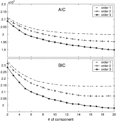
When the Fourier series approximation is used to cluster the periodic patterns of gene expression, two issues should be determined in the following sequence. First, what is the best order for Fourier series function that explains the time-dependent data? Second, what is the optimal number of components for the mixture model that each correspond to a different expression pattern? Model selection criteria, AIC and BIC, were used to determine the best Fourier series order and best number of mixture components for Spellman et al.’s data. The two criteria provide similar results (Figure 1), although our analysis is mostly based on BIC. It seems that a higher order of Fourier series can better fit time-dependent data than a lower order, reflecting the complexity of dynamic changes of gene expression. A lower order of Fourier series tends to detect a smaller number of gene-expression patterns than a higher order. For example, the first order detects 13 compo-nents, whereas the second and third orders detect 18 and .20 components, respectively. This makes sense because a higher order of Fourier series function has more power to discern subtle differences in gene-expression profiles. When closely looking at the BIC curves (Figure 1), the first order displays a dramatic decrease when the number of clusters is 6–8, whereas a dramatic decrease for the second and the third order occurs at 12–14 and 18–20 clusters, respectively.
To illustrate different periodic patterns of gene-expression profiles concordant with cell cycles, we used the first-order Fourier series to detect 13 patterns whose profiles (Figure 2) were drawn with the Fourier
param-eters estimated from the proposed model (Table 1). These 13 patterns differ dramatically in the overall shape of curves as defined by parameter sets ða0ˆ j;a1ˆ j;ˆb1j;TˆjÞ. On the basis of these estimates, a number of hypothesis tests can be made about the developmental patterns of gene expression. Table 1 also provides the estimates of the proportions of mixture components. The 13 patterns occur at different frequencies among the observed genes.
Computer simulation: We performed Monte Carlo simulation studies to investigate statistical properties of the functional clustering model proposed. A total of 1000 genes were simulated whose time-dependent expression was measured at 24 equally spaced time points. All the genes were sorted into three distinct patterns with varying proportions. The simulated gene-expression profiles follow an arbitrary form of periodic function. As has been mathematically clear, a periodic
Figure1.—Component number-dependent AIC and BIC
values of model fitting by a Fourier series function of order 1–3 for 800 genes collected from the yeast genome.
Figure2.—Thirteen periodic patterns of gene-expression
profiles approximated by a first-order Fourier series function for 800 genes collected from the yeast genome.
TABLE 1
MLEs of the Fourier parameters for 13 different periodic patterns of gene expression among 800 genes collected from
the yeast genome based on the first-order approximation
Pattern aˆ0j aˆ1j ˆb1j Tˆj vˆj
1 0.2888 0.9178 0.7847 10.47000 0.0151
2 0.0951 1.3955 0.0150 11.05000 0.0158
3 0.4384 0.0008 1.1269 9.96970 0.0371
4 0.0604 0.2396 1.2738 10.8740 0.0142
5 0.0382 0.0430 0.2508 2.0737 0.2309
6 0.0339 0.6301 0.1558 10.8620 0.0632
7 0.1277 0.1248 0.3128 9.6315 0.2011
8 0.1403 0.3256 0.5849 10.6880 0.0656
9 0.0177 0.5249 0.0052 10.5780 0.0667
10 0.2104 0.5480 0.0000 2.0006 0.0099
11 0.4395 3.1983 1.8160 8.2165 0.0013
12 0.0124 0.1115 0.1275 2.1848 0.1397
13 0.0359 0.0277 0.2932 2.0852 0.1394
function can be approximated by a Fourier series function. The Fourier parameters used for our simula-tion were assigned by values that are within their spaces according to Spellmanet al.’s (1998) data. The time-dependent covariance matrix of gene expression was structured by the AR(1) model. Different residual variances were used in the simulation to examine the effect of residual errors on parameter estimation.
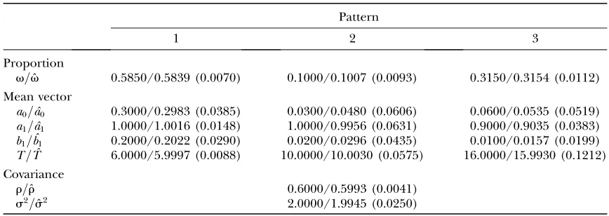
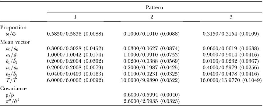
The optimal number of components for the simu-lated data was determined by calculating AIC and BIC values. As shown in Figure 3, the model can correctly estimate the number of components. On the basis of results from 1000 simulation replicates, the model can provide reasonably accurate and precise estimates of all Fourier parameters (Tables 2 and 3). The precision of parameter estimation depends on the proportion of a gene-expression pattern being better for a more fre-quent than for a less frefre-quent pattern. As expected, increasing residual variance will reduce the estimation precision of parameters (Table 2vs.Table 3). To show the robustness of the model, an additional simulation study based on a second-order Fourier series approxi-mation was performed. The results suggest that all parameters can be reasonably estimated even if the number of parameters being estimated is increased (Tables 4 and 5).
Nget al.(2006) proposed a random-effect mixture model for clustering gene-expression profiles through the incorporation of covariate information. When the covariate is time, Ng et al.’s model functions as ours does. However, these two models are different in three aspects. First, our model allows gene expres-sion measured at unevenly spaced time intervals and gene-specific differences in measurement schedule,
although these issues can be incorporated into Ng
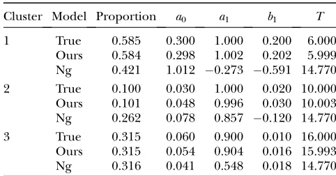
et al.’s model through extensive modifications. Second, we derived a closed form for the estimation of all the Fourier parameters for each gene cluster within the EM framework, whereas Nget al.estimated the period of the expression cycle for the mean Fourier curve of all genes by using the least-squares estimation approach. Third, our model is able and flexible enough to con-sider Fourier series approximation of any arbitrary order. We conducted an additional simulation exper-iment to compare the results from our and Nget al.’s models. The data from 1000 time-dependent gene expressions were simulated by assuming that these follow a multivariate normal distribution with gene cluster-specific mean vectors each fitted by a group of Fourier parameters and covariance matrix structured by the AR(1) model. Both our and Nget al.’s models can correctly estimate the number of gene clusters,i.e., three in this simulated example (Table 6). While our model is able to provide reasonably accurate estimates of the Fourier parameters, Nget al.’s model was quite biased for many parameter estimates. This comparative analysis suggests that our model will perform better than Ng et al.’s model when gene-expression profiles follow Fourier series approximations.
DISCUSSION
The use of microarray gene-expression technologies to understand developmental questions has received con-siderable attention in recent years (Panda et al.2002). Statistical approaches for analyzing time-dependent gene expression data have been proposed (Holteret al.2001;
Figure 3.—Component number-dependent
Qian et al. 2001; Bar-Joseph et al. 2003; Luan and Li2003; Parket al.2003; Wakefieldet al.2003; Ernst et al.2005; Storeyet al.2005; Maet al.2006; Nget al. 2006; Inoueet al.2007), but most of them are limited in both biological and statistical aspects. First, these approaches mostly based on a clustering analysis were not implemented with biological principles of gene expression that are related to a life process. For this reason, the results obtained from these approaches may not be biologically relevant and, thus, may be less useful for deciphering the developmental machinery of gene expression. The model proposed in this article integrates mathematical aspects of periodic gene expression into the analytical framework, thereby allowing for the interplay between gene expression and development.
Second, many existing approaches to clustering genes of a similar expression pattern on the basis of a
similarity measure have not considered the autocorre-lation of time series data and, therefore, fail to remove systematical measurement errors. Although some au-thors implemented time-dependent correlations into their models (e.g., Luanand Li2003; Nget al.2006), biological meanings of gene expression were not well considered. In the model proposed, the statistical principle of functional data analysis has been embed-ded into the model by structuring the time-dependent covariance matrix. This, on the one hand, de-noises repeated measurement errors and increases the effec-tiveness of the model and, on the other hand, enhances the model’s power due to a reduced number of parameters being estimated. As an illustration, we used a simple AR(1) model to approximate the covariance structure. Other models, such as a structured antede-pendence model (Zimmerman and Nu´ n˜ ez-Anto´ n 2001), can also be incorporated (see Jaffre´ zic et al.
TABLE 2
MLEs of the first-order Fourier parameters for three periodic patterns of gene expression among 1000 simulated genes with a given set of values (a0,a1,b1,T) under the residual variance ofs250.3
Pattern
1 2 3
Proportion
v=vˆ 0.5850/0.5851 (0.0002) 0.1000/0.1001 (0.0002) 0.3150/0.3148 (0.0005) Mean vector
a0=aˆ0 0.3000/0.30571 (0.0218) 0.0300/0.0511 (0.0378) 0.0600/0.0696 (0.0171)
a1=aˆ1 1.0000/1.0041 (0.0081) 1.0000/1.0007 (0.0081) 0.9000/0.9061 (0.0121)
b1=ˆb1 0.2000/0.1910 (0.0118) 0.0200/0.0084 (0.0141) 0.0100/0.0160 (0.0150)
T=Tˆ 6.0000/6.0034 (0.0043) 10.0000/10.0150 (0.0188) 16.0000/15.9730 (0.0392) Covariance
r=rˆ 0.6000/0.5888 (0.0044)
s2=sˆ2 0.3000/0.3013 (0.0036)
The averages of parameter estimates are calculated from 100 simulations and the mean square errors of the estimates are given in parentheses.
TABLE 3
MLEs of the first-order Fourier parameters for three periodic patterns of gene expression among 1000 simulated genes with a given set of values (a0,a1,b1,T) under the residual variance ofs252.0
Pattern
1 2 3
Proportion
v=vˆ 0.5850/0.5839 (0.0070) 0.1000/0.1007 (0.0093) 0.3150/0.3154 (0.0112)
Mean vector
a0=aˆ0 0.3000/0.2983 (0.0385) 0.0300/0.0480 (0.0606) 0.0600/0.0535 (0.0519)
a1=aˆ1 1.0000/1.0016 (0.0148) 1.0000/0.9956 (0.0631) 0.9000/0.9035 (0.0383)
b1=ˆb1 0.2000/0.2022 (0.0290) 0.0200/0.0296 (0.0435) 0.0100/0.0157 (0.0199)
T=Tˆ 6.0000/5.9997 (0.0088) 10.0000/10.0030 (0.0575) 16.0000/15.9930 (0.1212) Covariance
r=rˆ 0.6000/0.5993 (0.0041)
s2=sˆ2 2.0000/1.9945 (0.0250)
2003; Zhao et al. 2005), allowing the choice of an optimal model for structuring the covariance matrix. Finally, the mixture model-based approach allows for the estimation of the frequencies of various patterns of gene expression and the calculation of the posterior probability of each gene that belongs to a particular pattern.
The mixture-based approach incorporated by Fourier series approximation is a promising technique for detecting periodic gene-expression patterns. A major advantage of this approach lies in its remarkable flexibility to ask and address fundamental biological questions at the interplay between gene-expression and developmental patterns. Several important hypotheses
can be made from this approach, including those about the differences of gene expression in Fourier curve shapes, curve features, and duration of gene expression based on individual Fourier parameters that describe biological characteristics of periodic cycles. For example, the peak-to-trough ratio,am/bm, reflects the amplitude of expression profile and can be tested for its differences among the gene groups detected. If the mean curve is modeled with the Fourier series of order one,i.e.,
uðtÞ ¼a01a1cos 2pt
T
1b1sin 2pt
T
;
the hypothesis can be expressed as
TABLE 4
MLEs of the second-order Fourier parameters for three periodic patterns of gene expression among 1000 simulated genes with a given set of values (a0,a1,b1,T) under the residual variance ofs250.3
Pattern
1 2 3
Proportion
v=vˆ 0.5850/0.5850 (0.0004) 0.1000/0.1000 (0.0003) 0.3150/0.3150 (0.0003) Mean vector
a0=aˆ0 0.3000/0.2972 (0.0166) 0.0300/0.0340 (0.0291) 0.0600/0.0592 (0.0212)
a1=aˆ1 1.0000/1.0002 (0.0056) 1.0000/1.0018 (0.0169) 0.9000/0.8994 (0.0109)
b1=ˆb1 0.2000/0.1998 (0.0103) 0.0200/0.0211 (0.0214) 0.0100/0.0150 (0.0147)
a2=aˆ2 0.2000/0.2000 (0.0030) 0.2000/0.1997 (0.0112) 0.4000/0.3985 (0.0081)
b2=ˆb2 0.0400/0.0398 (0.0051) 0.0100/0.0121 (0.0103) 0.0400/0.0441 (0.0155)
T=Tˆ 6.0000/6.0002 (0.0030) 10.0000/10.0010 (0.0164) 16.0000/15.9880 (0.0397) Covariance
r=rˆ 0.6000/0.5998 (0.0044)
s2=sˆ2 0.3000/0.2995 (0.0039)
The averages of parameter estimates are calculated from 100 simulations and the mean square errors of the estimates are given in parentheses.
TABLE 5
MLEs of the second-order Fourier parameters for three periodic patterns of gene expression among 1000 simulated genes with a given set of values (a0,a1,b1,T) under the residual variance ofs252.6
Pattern
1 2 3
Proportion
v=vˆ 0.5850/0.5836 (0.0088) 0.1000/0.1010 (0.0088) 0.3150/0.3154 (0.0109) Mean vector
a0=aˆ0 0.3000/0.3028 (0.0452) 0.0300/0.0627 (0.0874) 0.0600/0.0619 (0.0638)
a1=aˆ1 1.0000/1.0042 (0.0174) 1.0000/0.9910 (0.0753) 0.9000/0.9014 (0.0416)
b1=ˆb1 0.2000/0.2004 (0.0302) 0.0200/0.0388 (0.0569) 0.0100/0.0232 (0.0367)
a2=aˆ2 0.2000/0.2008 (0.0079) 0.2000/0.1987 (0.0425) 0.4000/0.3979 (0.0256)
b2=ˆb2 0.0400/0.0409 (0.0163) 0.0100/0.0231 (0.0325) 0.0400/0.0478 (0.0416)
T=Tˆ 6.0000/6.0006 (0.0092) 10.0000/9.9890 (0.0522) 16.0000/15.9770 (0.1049) Covariance
r=rˆ 0.6000/0.5994 (0.0040)
s2=sˆ2 2.6000/2.5935 (0.0323)
H0: aj1=bj1[a1=b1 forj¼1;. . .;J
H1: at least one of the equalities above does not hold:
The slope of the gene expression profile may change with time, which suggests the occurrence of gene expression 3 time interaction effects during a time course. The differentiation ofu(t) with respect to timet
represents a slope of gene expression. If the slopes at a particular time pointt* are different between the curves of different gene groups, this means that significant gene expression3time interaction occurs between this time point and next. The test for gene expression 3 time interaction can be formulated with the hypotheses
H0:
d dt ujðt
*Þ ¼ d
dt uðt
*Þ vs: H 1:
d dt ujðt
*Þ 6¼ d
dtuðt
*Þ;
j¼1;. . .;k:
The effect of gene expression3time interaction can be examined during a given time course.
The new approach was used to analyze a real data set for periodic gene expression. The results from this approach suggest that it would be useful for the identification of gene clusters in terms of their periodic expression patterns. Through simulation studies, this approach has proved to provide reasonable accuracy and precision of parameter estimation and can be directly used to analyze a real data set of periodic gene expres-sion. This approach can be modified or extended in the following areas. First, the clustering and estimation of different gene-expression profiles depends on the pre-cise estimation of covariance functions. Fanet al.(2007b) proposed a semiparametric approach for modeling the covariance structure, which has been shown to be particularly powerful for functional data collected at irregular and subject-specific time points. The incorpo-ration of Fan et al.’s approach into our functional clustering model is expected to improve its power for
gene clustering. Second, when repeated measurement includes a high number of time points, the structuring of the covariance matrix may be quickly problematic. A handful of statistical models for dimension reduction proposed by J. Fan and his group (Fanet al.2007a; Fan and Lv2008) can be incorporated into our model, in a hope to increase the tractability of high-dimensional data. With these and other modifications, the approach for gene clustering presented in this article could be useful for addressing some development-relevant ques-tions in genetic control of complex biological processes. The computer code for the approach proposed in this article is available at statgen.ufl.edu.
We thank the two anonymous referees for their constructive comments on the manuscript, which led to significant improvement of its presentation. Part of this work was conducted when R. Wu spent his sabbatical leave at Princeton University. The preparation of this manuscript was partially supported by National Science Foundation grant no. 0540745 to R. Wu and the Brain Korea 21 project in 2007.
LITERATURE CITED
Akaike, H., 1974 A new look at the statistical model identification.
IEEE Trans. Automat. Contr.19:716–723.
Attinger, E. O., A. Anneand D. A. McDonald, 1966 Use of Fourier
series for the analysis of biological systems. Biophys. J.6:291–304. Bar-Joseph, Z., G. K. Gerber, D. K. Gifford, T. S. Jaakkolaand
I. Simon, 2003 Continuous representations of time-series gene
expression data. J. Comput. Biol.10:341–356.
Begum, E. A., B. Motoki, O. Makoto, Y. Hatsumi, K. Masatoshi
et al., 2006 Emergence of physiological rhythmicity in term
and preterm neonates in a neonatal intensive care unit. J. Circa-dian Rhythms4:11.
Carroll, R. J., and D. Ruppert, 1984 Power-transformations when
fitting theoretical models to data. J. Am. Stat. Assoc.79:321–328. Crosthwaite, S. K., 2004 Circadian clocks and natural antisense.
RNA FEBS Lett.567:49–54.
Dale, J. K., M. Maroto, M. L. Dequeant, P. Malapert, M. McGrew et al., 2003 Periodic notch inhibition by lunatic fringe underlies the chick segmentation clock. Nature421:275–278.
Davidian, M., and D. M. Giltinan, 1995 Nonlinear Models for
Re-peated Measurement Data.Chapman & Hall, London.
Durbin, J., 1967 Tests of serial independence based on the
cumu-lated periodogram. Bull. Int. Stat. Inst.42:1039–1049. Eisen, M. B., P. T. Spellman, P. O. Brown and D. Botstein,
1998 Cluster analysis and display of genome-wide expression patterns. Proc. Natl. Acad. Sci. USA95:14863–14868.
Ernst, J., G. J. Nauand Z. Bar-Joseph, 2005 Clsutering short time
series gene expression data. Bioinformatics21:i159–i168. Fan, J., and J. Lv, 2008 Sure independence screening for ultra-high
dimensional feature space (with discussion). J. R. Stat. Soc. Ser. B
70:849–911.
Fan, J., and Y. Ren, 2006 Statistical analysis of DNA microarray data
in cancer research. Clin. Cancer Res.12:4469–4473.
Fan, J., Y. Fanand J. Lv, 2007a High dimensional covariance matrix
estimation using a factor model. J. Econom (in press). Fan, J., T. Huangand R. Z. Li, 2007b Analysis of longitudinal data
with semiparametric estimation of covariance function. J. Am. Stat. Assoc.35:632–641.
Fraley, C., and A. E. Raftery, 1998 How many clusters? Which
cluster-ing method? Answers via model-based cluster analysis. Technical Re-port 329. Department of Statistics, University of Washington, Seattle. Frank, O., 1926 Die theorie der pulswellen. Zool. Biol.85:91–130.
Ghosh, D., and A. M. Chinnaiyan, 2002 Mixture modeling of gene
expression data from microarray experiments. Bioinformatics18:
275–286.
Glynn, E. F., J. Chen and A. R. Mushegian, 2006 Detecting
periodic patterns in unevenly spaced gene expression time series using Lomb-Scargle periodograms. Bioinformatics22:310–316.
TABLE 6
Comparisons between the results from our and NGet al.’s (2006) models for clustering time series gene-expression
profiles that are approximated by the first-order Fourier series
Cluster Model Proportion a0 a1 b1 T
1 True 0.585 0.300 1.000 0.200 6.000
Ours 0.584 0.298 1.002 0.202 5.999
Ng 0.421 1.012 0.273 0.591 14.770
2 True 0.100 0.030 1.000 0.020 10.000
Ours 0.101 0.048 0.996 0.030 10.003
Ng 0.262 0.078 0.857 0.120 14.770
3 True 0.315 0.060 0.900 0.010 16.000
Ours 0.315 0.054 0.904 0.016 15.993
Goldbeter, A., 2002 Computational approaches to cellular
rhythms. Nature420:238–245.
Gonze, D., J. Halloyand A. Goldbeter, 2002 Stochastic versus
de-terministic models for circadian rhythms. J. Biol. Phys.28:637–653. Gonze, D., J. Halloy, J. C. Leloupand A. Goldbeter, 2003 Stochastic
models for circadian rhythms: influence of molecular noise on pe-riodic and chaotic behavior. C. R. Biol.326:189–203.
Harmer, S. L., J. B. Hogenesch, M. Straume, H.-S. Chang, B. Han et al., 2000 Orchestrated transcription of key pathways in
Arabi-dopsisby the circadian clock. Science290:2110–2113.
Holter, N. S., A. Maritanand M. Cieplak, 2001 Dynamic modeling
of gene expression data. Proc. Natl. Acad. Sci. USA98:1693–1698. Inoue, L. Y., M. Neira, C. Nelson, M. Gleave and R. Etzioni,
2007 Cluster-based network model for time-course gene expres-sion data. Biostatistics8:507–525.
Jaffre´ zic, F., R. Thompsonand W. G. Hill, 2003 Structured
ante-dependence models for genetic analysis of multivariate repeated measures in quantitative traits. Genet. Res.82:55–65.
Kim, B.-R., R. C. Littelland R. L. Wu, 2006 Clustering the periodic
pattern of gene expression using Fourier series approximations. Curr. Genomics7:197–203.
Lakin-Thomas, P. L., and S. Brody, 2004 Circadian rhythms in
micro-organisms: new complexities. Annu. Rev. Microbiol.58:489–519. Leloup, J.-C., D. Gonzeand A. Goldbeter, 1999 Limit cycle
mod-els for circadian rhythms based on transcriptional regulation in Drosophila and Neurospora. J. Biol. Rhythms14:433–448. Luan, Y., and H. Li, 2003 Clustering of time-course gene expression
data using a mixed-effects model with B-splines. Bioinformatics
19:474–482.
Luan, Y., and H. Li, 2004 Model-based methods for identifying
pe-riodically expressed genes based on time course microarray gene expression data. Bioinformatics20:332–339.
Ma, P., C. I. Castillo-Davis, W. Zhongand J. S. Liu, 2006 A
data-driven clustering method for time course gene expression data. Nucleic Acids Res.34:1261–1269.
Mager, D. E., and D. R. Abernethy, 2007 Use of wavelet and fast
Fourier transforms in pharmacodynamics. J. Pharmacol. Exp. Ther.321:423–430.
McLachlan, G., and D. Peel, 2000 Finite Mixture Models.John Wiley
& Sons, New York.
McLachlan, G. J., R. W. Beanand D. Peel, 2002 A mixture
model-based approach to the clustering of microarray expression data. Bioinformatics18:414–422.
Mitchison, J. M., 2003 Growth during the cell cycle. Int. Rev. Cytol.
226:165–258.
Ng, S. K., G. J. McLachlan, K. Wang, L. B.-T. Jonesand S.-W. Ng,
2006 A mixture model with random-effects components for clustering correlated gene-expression profiles. Bioinformatics
22:1745–1752.
Panda, S., T. K. Sato, A. M. Castrucci, M. D. Rollag, W. J. DeGrip
et al., 2002 Melanopsin (Opn4) requirement for normal
light-induced circadian phase shifting. Science298:2213–2216.
Park, T., S. G. Yi, S. Lee, S. Y. Lee, D. H. Yooet al., 2003 Statistical
tests for identifying differentially expressed genes in time-course microarray experiments. Bioinformatics19:694–703.
Pletcher, S. D., and C. J. Geyer, 1999 The genetic analysis of
age-de-pendent traits: modeling a character process. Genetics153:825–835. Priestley, M. B., 1981 Spectral Analysis and Time Series. Academic
Press, San Diego.
Prolo, L. M., J. S. Takahashiand E. D. Herzog, 2005 Circadian
rhythm generation and entrainment in astrocytes. J. Neurosci.
25:404–408.
Qian, J., B. Stenger, C. A. Wilson, J. Lin, R. Jansen et al.,
2001 Partslist: a web-based system for dynamically ranking pro-tein folds based on disparate attributes, including whole-genome expression and interaction information. Nucleic Acids Res.29:
1750–1764.
Ramoni, M. F., P. Sebastianiand I. S. Kohane, 2002 Cluster analysis of
gene expression dynamics. Proc. Natl. Acad. Sci. USA99:9121–9126. Rovery, C., M. V. La, S. Robineau, K. Matsumoto, P. Renestoet al.,
2005 Preliminary transcriptional analsysis of spoT gene family and of membrane proteins inRickettsia conoriiandRickettsia felis.
Ann. NY Acad. Sci.1063:79–82.
Schwarz, G., 1978 Estimating the dimension of a model. Ann. Stat.
6:461–464.
Spellman, P. T., S. Sherlock, M. Q. Zhang, V. R. Iyer, K. Anerset al.,
1998 Comprehensive identification of cell cycle-regulated genes of the yeast Saccharomyces cerevisiae by microarray hybridization. Mol. Biol. Cell9:3273–3297.
Storey, J. D., W. Xiao, J. T. Leek, R. G. Tompkinsand R. W. Davis,
2005 Significant analysis of time course microarray experi-ments. Proc. Natl. Acad. Sci. USA102:12837–12842.
Verbeke, G., and G. Molenberghs, 2000 Linear Mixed Models for
Longitudinal Data.Springer-Verlag, New York.
Wakefield, J., C. Zhouand S. G. Self, 2003 Modelling gene
expres-sion data over time: curve clustering with informative prior distribu-tions, pp. 721–732 inBayesian Statistics 7,Proceedings of the Seventh Valencia International Meeting, edited by J. M. Bernardo, M. J.
Bayarri, J. O. Berger, A. P. Dawid, D. Heckerman, A. F. M. Smith
and M. West. Oxford University Press, London/New York/Oxford.
Wichert, S., K. Fokianosand K. Strimmer, 2004 Identifying
peri-odically expressed transcripts in microarray time series data. Bio-informatics20:5–20.
Wu, R. L., C.-X. Ma, M. Lin, Z. H. Wang and G. Casella,
2004 Functional mapping of quantitative trait loci underlying growth trajectories using a transform-both-sides logistic model. Biometrics60:729–738.
Zhao, W., Y. Q. Chen, G. Casella, J. M. Cheverudand R. L. Wu,
2005 A nonstationary model for functional mapping of com-plex traits. Bioinformatics21:2469–2477.
Zimmerman, D. L., and V. Nu´ n˜ ez-Anto´ n, 2001 Parametric modeling
of growth curve data: an overview (with discussion). Test10:1–73. Communicating editor: C. Haley
APPENDIX
In what follows, we derive the log-likelihood equations for estimating the unknown vectorV¼ ðfvj;Qujg
J j¼1;QvÞ.
The log-likelihood of parametersVconstructed on the basis of the mixture model is expressed as
logLðVjyÞ ¼X n
i¼1
log X
J
j¼1
vjfijðyi;Quj;QvÞ
" #
;
and the posterior probability with which theith gene belongs to the jth pattern is defined by Equation 4. Since vJ ¼1PJj¼11vj, we have
@logLðVjyÞ
@vj
¼X n
i¼1
fijðyi;Quj;QvÞ fJðyi;Quj;QvÞ
PJ
j9¼1vj9fj9ðyi;Quj;QvÞ
¼X n
i¼1
Pij vj
PiJ 1PJj¼11vj
" #
By setting it equal to zero, we have
ˆ vj ¼
Pn i¼1Pij Pn
i¼1PiJ
1X
J1
j¼1 vj " #
: ðA1Þ
By plugging in ˆvj into the right side of Equation A1, we have
ˆ vj ¼
Pn
i¼1Pij=Pni¼1PiJ 11PJj¼11ðPn
i¼1Pij= Pn
i¼1PiJÞ
¼
Pn
i¼1Pij=Pni¼1PiJ 11PJj¼11Pn
i¼1Pij=Pni¼1PiJ ¼
Pn
i¼1Pij=Pni¼1PiJ 11Pn
i¼1 PJ1
j¼1Pij=Pni¼1PiJ ¼
Pn i¼1Pij Pn
i¼1PiJ1 Pni¼1 PJ1
j¼1Pij
¼
Pn i¼1Pij Pn
i¼1ðPiJ1 PJ
1 j¼1 PijÞ
¼ Pn
i¼1Pij
n : ðA2Þ
Assuming that the model is implemented by a first-order Fourier series approximation, unknown Fourier parameters are specified asQuj ¼ ðcj;TjÞ, wherecj5(a0j,a1j,b1j). We have
@logLðVjyÞ
@cj ¼
@logLðVjyÞ
@uij
@
uij
@cj
:
Note that
@logLðVjyÞ
@uij ¼ Xn
i¼1
vjð@fijðyi;Quj;QvÞ=@uijÞ
PJ
j9¼1vj9fj9ðyi;Quj;QvÞ
¼X n
i¼1
vjfijðyi;Quj;QvÞ
PJ
j9¼1vj9fj9ðyi;Quj;QvÞ
ðyiuijÞ9Si1
¼X n
i¼1
PijðyiuijÞ9Si1:
Let
FiðTjÞ ¼
1 cos 2pti1 Tj
sin 2pti1 Tj
1 cos 2pti2 Tj
sin 2pti2 Tj
.. .
.. .
.. .
1 cos 2ptiTi Tj
sin 2ptiTi Tj
0 B B B B B B B B @
1 C C C C C C C C A
Ti33
;
and then we have
uij¼FiðTjÞcjand@uij cj
¼FiðTjÞ:
@logLðVjyÞ
@cj ¼ Xn
i¼1
PijðyiuijÞ9S1
i FiðTjÞ ¼ set
0;
which leads to
Xn
i¼1
Piju9ijSi1FiðTjÞ ¼ Xn
i¼1
Pijy9iSi1FiðTjÞ:
We further have
Xn
i¼1
Pijc9jFiðTjÞ9Si1FiðTjÞ ¼ Xn
i¼1
Pijy9iSi1FiðTjÞ:
IfPijFiðTjÞ9S
1
i FiðTjÞis invertable, we have
ˆc9j ¼ ðaˆ0j;aˆ1j;ˆb1jÞ
¼ X n
i¼1
Pijy9iSi1FiðTjÞ
" #
Xn
i¼1
PijFiðTjÞ9S1FiðTjÞ " #1
: ðA3Þ
Note thatfijðyi;Quj;QvÞcan be written as
fijðyi;Quj;QvÞ ¼
1 ð2pÞTi=2ðs2ÞTi=2jR
ij1=2
exp 1
2s2ðyiuijÞ9Ri1ðyiuijÞ
" #
:
If we writeSi¼s2Ri, where
Ri ¼
1 r r2 . . . rtiTi1
r 1 r . . . rtiTi2
.. .
.. .
.. .
rtiTi1 rtiTi2 rtiTi3 . . . 1
0 B B B @
1 C C C A
Ti3Ti
;
we have
@fijðyi;Quj;QvÞ
@s2 ¼ 1
2s2 fijðyi;Quj;QvÞ
ðyiuijÞ9Ri1ðyiuijÞ
s2 Ti
and
@logLðVjyÞ
@s2 ¼ Xn
i¼1 XJ
j¼1
vj PJ
j9¼1vj9fj9ðyi;Quj;QvÞ
@fijðyi;Quj;QvÞ
@s2
¼X n
i¼1 XJ
j9¼1
Pij 2s2
ðyiuijÞ9Ri1ðyiuijÞ
s2 Ti
¼ set
0:
By solving it fors2, we have
Tis2 Xn
i¼1 XJ
j¼1
Pij¼ Xn
i¼1 XJ
j¼1
PijðyiuijÞ9Ri1ðyiuijÞ;
so
ˆ s2 ¼
Pn i¼1
PJ
j¼1PijðyiuijÞ9R
1
i ðyiuijÞ
TiPni¼1 PJ
j¼1Pij ¼
Pn i¼1
PJ
j¼1PijðyiuijÞ9Ri1ðyiuijÞ
Tin
For the AR(1) model, we have
Ri1¼ 1 1r2
1 r 0 0 0 . . . 0
r 11r2 r 0 0 . . . . . . . . . 0
0 r 11r2 r 0 . . . 0
.. . .. . .. . .. . .. . .. . .. . .. . .. .
0 0 0 0 0 . . . r 11r2 r
0 0 0 0 0 . . . r 1
0 B B B B B B B B B B B @ 1 C C C C C C C C C C C A
Ti3Ti
;
and
jRji¼ ð1r2ÞTi1: Let
mij¼yiuij and mijðtitÞ ¼yiðtitÞ uijðtitÞ:
Then, we have
@½ð1=2s2ÞðyiuijÞ9Ri1ðyiuijÞ
@r
¼@½ð1=2s 2Þm9
ijRi1mij
@r
¼ @
@r 1 2s2ð1r2Þ
XTi
t¼1
m2ijðtitÞ 2r
X Ti1 t¼1
mijðtitÞmijðtit11Þ1r2
X Ti1
t¼2 m2ijðtitÞ
( )
" #
¼ 1 s2ð1r2Þ
1 1r2 m9ijR
1 i mij1r
X Ti1
t¼2
m2ijðtitÞ
X Ti1
t¼1
mijðtitÞmijðtit11Þ
" #
;
and
@fijðyi;Quj;QvÞ
@r
¼ðTi1Þr
ð1r2Þ fijðyi;Quj;QvÞ1fijðyi;Quj;QvÞ
@½ð1=2s2Þðy
iuijÞ9Ri1ðyiuijÞ @r
¼fijðyi;Quj;QvÞ
3 ðTi1Þr ð1r2Þ
1 s2ð1r2Þ
1 1r2m9ijR
1
i mij1r X Ti1
t¼2
m2
ijðtitÞ
X Ti1
t¼1
mijðtitÞmijðtit11Þ
( )
" #
:
Therefore, we have
@logLðVjyÞ
@r
¼X n
i¼1 XJ
j¼1
vj PJ
j9¼1vj9fj9ðyi;Quj;QvÞ
@fijðyi;Quj;QvÞ
@r
¼X n
i¼1 XJ
j¼1
Pij
fijðyi;Quj;QvÞ
@fijðyi;Quj;QvÞ
@r
¼X n
i¼1 XJ
j¼1
Pij 1r2
3 ðTi1Þr 1 s2
1 1r2 m9ijR
1 i mij1r
X Ti2
t¼2
m2ijðtitÞ
X Ti1
t¼1
mijðtitÞmijðtit11Þ
( )
" #
¼ set
By solving the above log-likelihood equation, the MLE ofrcan be obtained as
r
ˆ¼ Pn
i¼1 PJ
j¼1Pij ð1=ð1r2ÞÞm9ijRi1mij1r PTi1
t¼2 m2ijðtitÞ PTt¼i11mijðtitÞmijðtit11Þ
h i
s2ðr1ÞPn i¼1
PJ j¼1Pij
¼ Pn
i¼1 PJ
j¼1Pij ð1=ð1r2ÞÞm9ijRi1mij1r PTi1
t¼2 m2ijðtitÞ Pt¼Ti11mijðtitÞmijðtit11Þ
h i
nðTi1Þs2
: ðA5Þ