ABSTRACT
MOON, CHANGSUNG. Predictive Modeling of Complex Graphs as Context and Semantics Preserving Vector Spaces. (Under the direction of Dr. Nagiza F. Samatova.)
Predictive modeling of complex graphs is a process that uses complex graph data and probability theory to forecast outcomes. Relational data, such as social networks and knowledge bases, can be represented as complex graphs with directed, multi-edge relationships, including self-loops. These graphs can also have a homogeneous or heterogeneous set of vertex and edge types. The main challenges with predictive modeling of complex graphs are improving scalability for large data and improving prediction accuracy, such as finding missing vertices, which can be done by analyzing the context and semantic information of the graphs. The context information can be represented as a group of vertices that have frequently appeared near each other in a sequence graph, while the semantic information can be represented by edge types among the vertices. Most graph modeling methods that directly extract this information from observed edges have scalability limitations. In such scenarios, we hypothesize that vector embedding (i.e., vector representation) methods can be developed to find representational vector spaces to model complex graphs in such a way that context and semantic information is preserved. These methods enable the predictive modeling of complex graphs in fixed low-dimensional vector spaces. Recently, vector space embedding methods of various tasks of predictive analysis, such as finding a missing word in a sentence, have been gaining considerable attention in big data analysis because of their notable improvement in scalability by representing features in a low-dimensional vector space.
This work initially addresses two research challenges with regards to predictive analysis in complex graphs: 1) automatic completion of user-intended actions and 2) automatic knowledge graph (KG) completion, i.e., inference of missing entities as well as missing relationship and entity types in a knowledge graph, which is a multi-relational graph that has a heterogeneous set of vertex and edge types. Accurate and efficient prediction of future user actions is a challenging task as user action data, represented as a sequence of actions such as (
Access_flight_booking_website
,Search_for_flights
,Purchase_flight
,Board_flight
, ...) and a single-relational graph that has a homogeneous set of vertex and edge types, does not capture relationships among actions. Moreover, KGs, which consist of entities (e.g.,Barack_Obama
andHawaii
) and relation types (e.g.,bornIn
) between them, are plagued by numerous missing entities and relation types. Hence, the task of KG completion, in which we are looking to infer missing entities and relation types, is particularly challenging. Any missing data can reduce the power of a model, lead to a biased model, or lead to incorrect predictions.predictive strength, they have issues capturing semantic relationships among actions. In the task of KG completion, latent embedding methods, which automatically infer latent features from data, have shown notable results. However, most existing methods only consider the relationship in triples (subject, predicate, object), even though capturing relationships among relation types can improve the prediction accuracy.
In this dissertation, we seek to improve both prediction of user actions and KG completion by inventing vector space embedding methods. We first propose an online method, Frequency Vector (FVEC) prediction, that predicts next actions by combining scores from our new models: a frequency analysis model and a vector embedding model. The frequency model captures the frequency of sequential patterns, which is critical context information for inferring next actions, while the embedding model can deal with new actions preserve context information in a vector space and capture semantic relationships among actions. In the experiments, FVEC had a consistently higher accuracy (up to 4.68%) and a lower standard deviation than all tested online methods.
For the prediction of missing entities and relation types in KGs, we present a contextual embed-ding method CONTE that learns the vector embeddings of entities and relation types while taking contextual relation typesinto account. Contextual relation types consist of the surrounding relation types of a triple, and they can be used to capture relationships among relation types. We show that by taking these relation types into account, we can improve the prediction accuracy by an average of 14% against state-of-the-art methods.
© Copyright 2018 by Changsung Moon
Predictive Modeling of Complex Graphs as Context and Semantics Preserving Vector Spaces
by
Changsung Moon
A dissertation submitted to the Graduate Faculty of North Carolina State University
in partial fulfillment of the requirements for the Degree of
Doctor of Philosophy
Computer Science
Raleigh, North Carolina 2018
APPROVED BY:
Dr. Dennis R. Bahler Dr. Ranga R. Vatsavai
Dr. Steffen Heber Dr. Nagiza F. Samatova
BIOGRAPHY
ACKNOWLEDGEMENTS
First and foremost, I would like to thank my advisor, Dr. Nagiza Samatova, for her expert guidance, ideas and motivating feedback over the years. I am very grateful to my committee members, Dr. Dennis Bahler, Dr. Ranga Vatsavai, and Dr. Steffen Heber, for their valuable time and feedback. I would also like to thank graduate students in the Dr. Samatova’s research group, especially Paul Jones, Steve Harenberg, Shiou Tian Hsu and Dakota Medd, who provided helpful feedback for my research and for the associated publications. I have had the pleasure of collaborating with researchers at the Laboratory for Analytic Sciences (LAS), especially Matthew Schmidt and John Slankas. Finally, many thanks to my father, Jongsik Moon, my mother, Haesoon Oh, my wife, Dongwha Sohn, and my kids, Ryan and Ellie, for their unconditional love and support.
TABLE OF CONTENTS
LIST OF TABLES . . . vi
LIST OF FIGURES. . . vii
Chapter 1 INTRODUCTION . . . 1
1.1 Motivation . . . 1
1.2 Background . . . 5
1.2.1 Embeddings . . . 5
1.2.2 Optimization Approaches . . . 7
1.2.3 Batch and Online Learning . . . 11
1.3 Research Questions and Approaches . . . 12
1.3.1 Predicting User’s Next Actions . . . 12
1.3.2 Inferring Missing Entities and Relation Types . . . 13
1.3.3 Inferring Missing Entity Types . . . 13
1.4 Publications . . . 14
1.4.1 Published . . . 14
1.4.2 Accepted . . . 15
Chapter 2 ONLINE PREDICTION OF USER ACTIONS . . . 16
2.1 Introduction . . . 16
2.2 Problem Definition . . . 17
2.3 Background . . . 19
2.4 Method . . . 20
2.4.1 Frequency Model . . . 20
2.4.2 Vector Model . . . 21
2.4.3 Prediction . . . 26
2.4.4 Updating the Vector Model . . . 26
2.5 Empirical Evaluation . . . 27
2.5.1 Datasets . . . 27
2.5.2 Baseline Methods . . . 28
2.5.3 Training, Validation and Test Sets . . . 31
2.5.4 Selecting Parameters for FVEC . . . 33
2.5.5 Experimental Results . . . 35
2.6 Summary . . . 39
Chapter 3 INFERRING MISSING ENTITIES AND RELATION TYPES . . . 40
3.1 Introduction . . . 40
3.2 Problem Definition . . . 42
3.3 Related Work . . . 43
3.3.1 Translating Embeddings . . . 43
3.3.2 Other Models . . . 44
3.4 Method . . . 45
3.4.2 Margin-Based Ranking Loss Function . . . 47
3.4.3 Optimization . . . 48
3.4.4 Prediction . . . 49
3.5 Empirical Evaluation . . . 50
3.5.1 Datasets . . . 50
3.5.2 Baseline Methods and Implementation . . . 51
3.5.3 Parameter Selection . . . 53
3.5.4 Experimental Results . . . 54
3.6 Summary . . . 58
Chapter 4 INFERRING MISSING ENTITY TYPES . . . 59
4.1 Introduction . . . 59
4.2 Problem Statement . . . 60
4.3 Method . . . 62
4.3.1 Learning Embeddings of Entity Types . . . 63
4.3.2 Negative Sampling . . . 65
4.3.3 Margin-Based Ranking Loss Function . . . 66
4.3.4 Prediction . . . 66
4.4 Empirical Evaluation . . . 69
4.4.1 Datasets . . . 69
4.4.2 Baseline Methods . . . 69
4.4.3 Parameter Selection . . . 71
4.4.4 Experimental Results . . . 71
4.5 Summary . . . 73
Chapter 5 CONCLUSION AND FUTURE WORK . . . 74
5.1 Conclusion . . . 74
5.2 Future Work . . . 75
LIST OF TABLES
Table 2.1 Notations . . . 18
Table 2.2 Number of Unique Actions . . . 35
Table 2.3 Top 1 and 3 Prediction Accuracy over UDC dataset. All are % values exceptn and|As e e n|. . . 38
Table 2.4 Top 1 and 3 Prediction Accuracy over Word dataset. All are % values exceptn and|As e e n|. . . 39
Table 2.5 Top 1 and 3 Prediction Accuracy over Reality Mining dataset. All are % values exceptnand|As e e n|. . . 39
Table 3.1 Memory Complexity of Embedding Models (ne: # of entities,nr: # of relation types,nm: # of projection matrices of all sub-types, andk: # of dimensions) . . 45
Table 3.2 Statistics of Datasets . . . 49
Table 3.3 Relation Type Prediction Accuracy on FB15k . . . 54
Table 3.4 Relation Type Prediction Accuracy on YAGO43k . . . 54
Table 3.5 Entity Prediction Accuracy on FB15k . . . 55
Table 3.6 Entity Prediction Accuracy on YAGO43k . . . 55
Table 4.1 Samples of Clustered Entities on YAGO43k . . . 64
Table 4.2 Characterization of Datasets. We create two additional datasets (derived from FB15k and YAGO43k) that include entity types. These are denoted with a ET suffix. . . 67
Table 4.3 Entity Type Prediction Accuracy on FB15kET . . . 72
LIST OF FIGURES
Figure 1.1 Example of a Single-Relational Directed Graph . . . 2
Figure 1.2 Example of a Multi-Relational Directed Graph . . . 2
Figure 1.3 An Example of A Sequence of User Actions and Predictions for Next Actions . 3 Figure 1.4 An Example of an Entity in the Knowledge Graph YAGO . . . 4
Figure 1.5 The Number of Person Entities in DBpedia . . . 5
Figure 1.6 Example of Word Embeddings in Two Dimensions . . . 6
Figure 1.7 An Example of Generating a Knowledge Graph from Real-World Input Docu-ments that have Missing Facts . . . 7
Figure 1.8 Illustration of the Knowledge Graph from Figure 1.7 Enriched with Additional Inferred Relationships, which may be generated either by a Human Analyst or by an Algorithm such as those presented in this Dissertation. . . 8
Figure 1.9 Stochastic Gradient Descent Fluctuations in the Objective Function as Gradi-ent Steps (Source: Wikipedia) . . . 9
Figure 2.1 CBOW neural network architecture . . . 19
Figure 2.2 Example trie structure created by FVEC . . . 21
Figure 2.3 Sliding a Window for the Vector Model . . . 22
Figure 2.4 Vector Model between Input layer and Hidden layer . . . 23
Figure 2.5 An example Huffman tree used in our Modified Hierarchical Softmax . . . 23
Figure 2.6 FVEC neural network architecture . . . 24
Figure 2.7 Prediction . . . 26
Figure 2.8 Changes of The Learning Rateηt r a i n i n g . . . 27
Figure 2.9 Top-1,3 accuracy whenβ=0. Optimizing the value oflc using UDC, Word and Reality Mining validation datasets with 7900, 1900 and 1900 training respectively and 100 validation samples. . . 29
Figure 2.10 Top-1,3 accuracy whenβ=1. Optimizing the value oflc using UDC, Word and Reality Mining validation datasets with 7900, 1900 and 1900 training respectively and 100 validation samples. . . 29
Figure 2.11 Top-1 accuracy whenlc =5 for the frequency model andlc=2 for the vec-tor model. Optimizing the value ofβ using UDC, Word and Reality Mining validation datasets with 7900, 1900 and 1900 training respectively and 100 validation samples. . . 30
Figure 2.12 Top-3 accuracy whenlc =5 for the frequency model andlc=2 for the vec-tor model. Optimizing the value ofβ using UDC, Word and Reality Mining validation datasets with 7900, 1900 and 1900 training respectively and 100 validation samples. . . 30
Figure 2.13 Top-1 accuracy for UDC dataset with various test sizes . . . 32
Figure 2.14 Top-3 accuracy for UDC dataset with various test sizes . . . 32
Figure 2.15 Creating Training and Test Sets . . . 33
Figure 2.16 Top-1 standard deviation for UDC dataset with various test sizes . . . 34
Figure 2.17 Top-3 standard deviation for UDC dataset with various test sizes . . . 34
Figure 2.19 Top-N accuracy for UDC dataset . . . 37
Figure 2.20 Top-N accuracy for Word dataset . . . 37
Figure 2.21 Top-N accuracy for Reality Mining dataset . . . 38
Figure 3.1 Sample Knowledge Graph. Figure adapted from[Nic16a]. . . 41
Figure 3.2 Contextual Relation Types for a Triple(s,p,o)in a KG . . . 42
Figure 3.3 An example of the steps involved in computing the Mean Reciprocal Rank (MRR). In this case the mean of the reciprocal ranks is≈0.61. . . 43
Figure 3.4 A framework for learning vectors of entities and relation types . . . 47
Figure 3.5 MRR of Relation Type Prediction for the FB15k Validation Dataset . . . 51
Figure 3.6 MRR of Relation Type Prediction for the YAGO43k Validation Dataset . . . 51
Figure 3.7 MRR of Entity Prediction for the FB15k Validation Dataset . . . 52
Figure 3.8 MRR of Entity Prediction for the YAGO43k Validation Dataset . . . 52
Figure 3.9 TRANSE: A t-SNE plot of relation types with 9 high-level classes (Red: educa-tion, Blue: film, Black: geography, Orange: tv, Green: sports, Purple: music, Brown: location, Yellow: medicine, Magenta: government) . . . 56
Figure 3.10 HOLE: A t-SNE plot of relation types with 9 high-level classes (Red: education, Blue: film, Black: geography, Orange: tv, Green: sports, Purple: music, Brown: location, Yellow: medicine, Magenta: government) . . . 56
Figure 3.11 CONTE: A t-SNE plot of relation types with 9 high-level classes (Red: education, Blue: film, Black: geography, Orange: tv, Green: sports, Purple: music, Brown: location, Yellow: medicine, Magenta: government) . . . 57
Figure 4.1 Entity types for ‘Michael_Jordan’ from the YAGO knowledge graph . . . 61
Figure 4.2 A t-SNE plot of entities with an entity type (Red:/education/ educational_-institution, Blue: /film/film, Purple: /tv/tv_actor, Orange: /book/author, Green:/tv/tv_program, Black:/music/instrument) . . . 62
Figure 4.3 A pipeline of ETE (Blue: input dataset, Yellow: method, Gray: output) . . . 65
Figure 4.4 A framework for learning vectors of entity types . . . 66
Figure 4.5 MRR of Entity Type Prediction of ETE and the Extended Baselines for the FB15kET Validation Dataset . . . 67
Figure 4.6 MRR of Entity Type Prediction of ETE and the Extended Baselines for the YAGO43kET Validation Dataset . . . 68
Figure 4.7 MRR of Entity Type Prediction of the Original Baselines for the FB15kET Validation Dataset . . . 68
CHAPTER
1
INTRODUCTION
1.1
Motivation
1
Article A
Article B
Article C
Article D
Article E
Article F
Figure 1.1Example of a Single-Relational Directed Graph
1 Article A
Article B
Person C
Article D
Article E
Person F cites
authored
authored
reviewed cites
cites
authored
Figure 1.2Example of a Multi-Relational Directed Graph
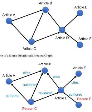
pair of vertices. Although the size of KGs can be huge, KGs often suffer from an abundance of missing information. KG completion is the task of inferring missing information by analyzing the semantic information in the graph. Figure 1.1 and 1.2 show examples of a single-relational graph and a multi-relational graph respectively. In the first example, the single-relational graph has a homogeneous set of vertices (i.e. they all representArticles) and of edge types (representing the relation ’cites’). The multi-relational graph has a heterogeneous set of vertices (ArticlesandPersons) and edge types (cites,reviewedandauthored). In this dissertation, we focus on learning predictive models based on these two kinds of complex graphs.
Figure 1.3An Example of A Sequence of User Actions and Predictions for Next Actions
observed edges have limited scalability. To address this issue, we propose vector embedding (i.e., vector representation) methods to find representational vector spaces to model complex graphs while preserving context and semantic information. These methods enable predictive modeling of complex graphs in fixed low-dimensional vector spaces. Recently, vector space embedding methods for various tasks of predictive analysis have been gaining considerable attention in big data analysis because of their notable improvement in scalability by representing features in a low-dimensional vector space.
In this dissertation, we address two research challenges with regards to predictive analysis in complex graphs: 1) automatic completion of user-intended actions and 2) automatic knowledge graph (KG) completion; i.e., inference of missing entities as well as missing relationship and entity types in a knowledge graph.
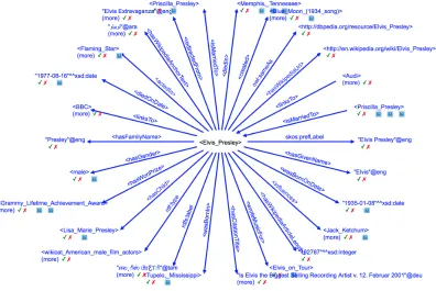
Figure 1.4An Example of an Entity in the Knowledge Graph YAGO
after
Pages
.0 500,000 1,000,000 1,500,000 2,000,000 2,500,000 3,000,000 3,500,000
2012-06 2013-04 2014-06 2015-04 2015-10 2016-04
Figure 1.5The Number of Person Entities in DBpedia
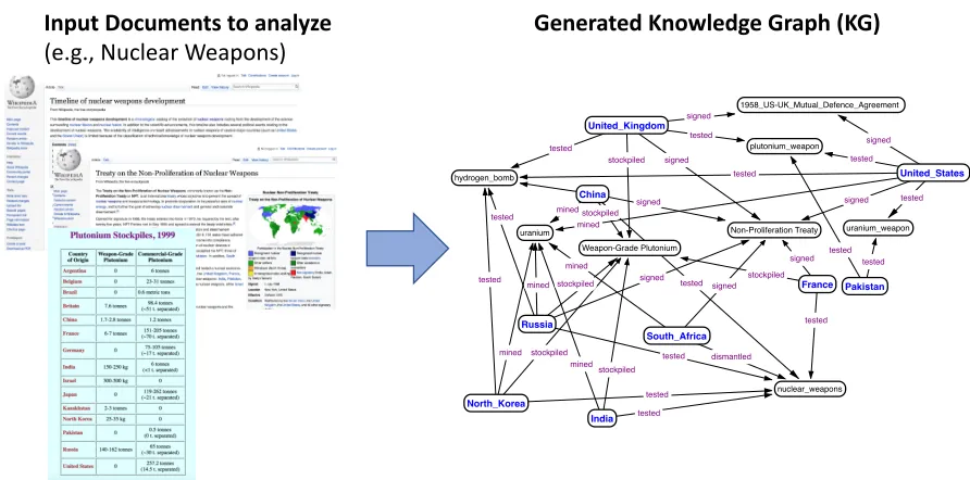
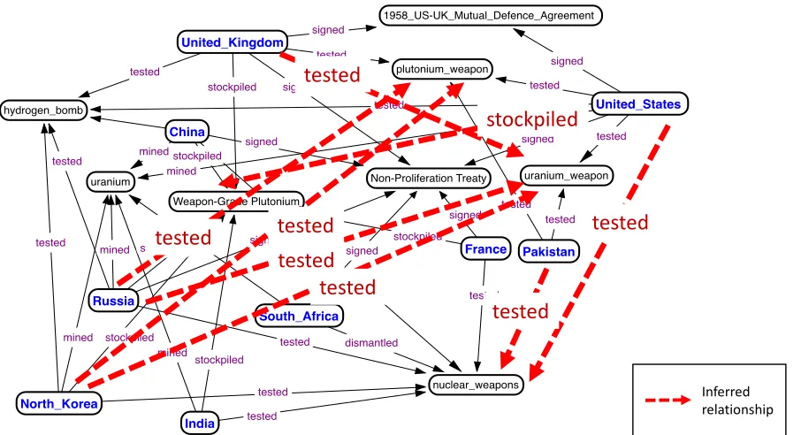
will often, either deliberately or unintentionally, omit certain facts related to the document topic (for instance, if they are considered to be self-evident or unnecessary). Therefore, if we generate a graph from documents that have missing facts, we would naturally expect the corresponding knowledge graph to also have missing vertices and edges. The right hand graphic in Figure 1.7 shows a generated graph from documents relating to nuclear weapons. Vertices represent countries, weapons, etc, and edge labels indicate relationships between vertices such as tested, stockpiled, etc. Figure 1.8 shows an enriched version of this graph. Missing facts (or at least educated guesses) can be discovered by inferring missing relationships in the knowledge graph. Recently, knowledge graph embedding methods have shown good results on this inference problem. The enriched knowledge graph can subsequently be used for more accurate analysis of the domain. Such missing data can reduce the power of a model or can lead to a biased model. It can also lead to erroneous predictions or classifications. The task ofknowledge graph completionis to infer missing entities, entity types and relation types.
1.2
Background
1.2.1 Embeddings
Figure 1.6Example of Word Embeddings in Two Dimensions
relationships. For example, in NLP, these models often represent words in a continuous vector space and map semantically similar words to nearby points[Mik13b]. We call these vector representations the “embedding" because they are not directly observed in the data; rather, they are learned from the training data. Word embeddings that incorporate semantic relationships could be used to improve performance in many NLP applications, such as machine translation, information retrieval and question-answering systems.
Before we start describing our approaches, we would like to explain some details about word embeddings. There are many ways to represent a word. One of the most popular approaches is a one-hot encoding, where each word has a 1 in a unique bit-position, and a 0 at all other locations in an array. The size of the one-hot encoding vector is the same as the size of the vocabulary. This approach is simple, but we cannot discover the relationship between words from these vectors. There are also problems related to sparsity and inefficient memory usage with this approach. Suppose you have 1, 000, 000 words in your vocabulary, and each word is represented as a 1, 000, 000-dimensional vector. You would have to deal with a big sparse matrix that is 1, 000, 000×1, 000, 000. This sparse representation would not be efficient with such a large vocabulary.
1 United_States uranium_weapon plutonium_weapon 1958_US-UK_Mutual_Defence_Agreement United_Kingdom hydrogen_bomb nuclear_weapons France South_Africa Russia China uranium India North_Korea Pakistan Non-Proliferation Treaty Weapon-Grade Plutonium mined mined mined mined mined mined signed signed tested tested tested tested tested dismantled tested tested tested signed signed signed signed signed signed tested tested tested tested stockpiled stockpiled stockpiled stockpiled tested stockpiled stockpiled tested
Input Documents to analyze
(e.g., Nuclear Weapons)
Generated Knowledge Graph (KG)
Figure 1.7An Example of Generating a Knowledge Graph from Real-World Input Documents that have Missing Facts
model has learned word embeddings, they can be reused efficiently in a variety of NLP applications. In practice, instead of training word embeddings from scratch, we can typically download pre-trained word embeddings and use them in NLP applications.
1.2.2 Optimization Approaches
We use Gradient Descent as our optimization algorithm. The general idea of Gradient Descent is to tweak parametersθiteratively in order to minimize a cost function by measuring the gradient of the cost function with regards to the parameters. First of all, the parameters can be initialized with random values, and then we update them gradually one step at a time. At each step, we decrease the cost function until it converges to a minimum.
1 United_States uranium_weapon plutonium_weapon 1958_US-UK_Mutual_Defence_Agreement United_Kingdom hydrogen_bomb nuclear_weapons France South_Africa Russia China uranium India North_Korea Pakistan Non-Proliferation Treaty Weapon-Grade Plutonium mined mined mined mined mined mined signed signed tested tested tested tested tested dismantled tested tested tested signed signed signed signed signed signed tested tested tested tested stockpiled stockpiled stockpiled stockpiled tested stockpiled stockpiled tested
tested
tested
tested
tested
tested
tested
stockpiled
tested
Inferred relationshipFigure 1.8Illustration of the Knowledge Graph from Figure 1.7 Enriched with Additional Inferred Relation-ships, which may be generated either by a Human Analyst or by an Algorithm such as those presented in this Dissertation.
1.2.2.1 Batch Gradient Descent
Batch Gradient Descent computes the gradient of the cost function with regards to the parameters θfor the entire observations as follows:
θ=θ−η· ∇θJ(θ) (1.1)
whereηis the learning rate, andJ(θ)is the cost function. This approach requires looking at all observations to perform just one update. Batch Gradient Descent is guaranteed to converge to the global minimum for a convex error surface and to the local minimum for a non-convex error surface. However, the main disadvantage of Batch Gradient Descent is that it is very slow with a large dataset and therefore is not suitable for use with online models.
1.2.2.2 Stochastic Gradient Descent
Figure 1.9Stochastic Gradient Descent Fluctuations in the Objective Function as Gradient Steps (Source: Wikipedia)
θ=θ−η· ∇θJ(θ;x(i);y(i)) (1.2)
This approach usually works much faster than Batch Gradient Descent because it does not require all the observations to perform each update. This means that, Stochastic Gradient Descent typically allows us to update a model online. Generally, knowledge graphs and user behavior datasets are huge and dynamic, so Stochastic Gradient Descent could be a good fit for these kinds of data. We apply this approach in our research. However, this gradient descent method performs frequent updates with a high variance that cause the loss function to fluctuate as shown in Figure 1.9, while Batch Gradient Descent tends to converge to the minimum smoothly. Indeed, SGD can fluctuate around the minimum and might not converge to the minimum at all. Conversely, Stochastic Gradient Descent is able to jump to new and better local or global minima. We can improve SGD by decreasing the learning rateηover time. SGD converges to the global minimum for a convex error surface and to the local minimum for a non-convex error surface.
1.2.2.3 Mini-batch Gradient Descent
Mini-batch Gradient Descent performs an update for every mini-batch ofnobservations as follows:
θ=θ−η· ∇θJ(θ;x(i:i+n);y(i:i+n)) (1.3)
called mini-batches instead of computing the gradients based on all observations or based on just one observation. This approach reduces the variance of the parameter updates and can get a performance boost in a distributed computing environment. The common mini-batch sizes range between 50 and 256, but can vary for different applications.
1.2.2.4 AdaGrad[Duc11]
AdaGrad adapts the learning rateηto the parametersθ by performing larger updates for infrequent parameters and smaller updates for frequent parameters. This ensures that this approach works well with sparse data such as knowledge graphs. Knowledge graphs are very sparse when it comes to connections between entities. For this reason, we applied Stochastic Gradient Descent with AdaGrad to our knowledge graph completion methods. AdaGrad updates every parameterθiat every time stept as follows:
θt+1,i=θt,i−η· ∇θJ(θi) (1.4) and then, this approach modifies the learning rateηat each time stept based on the past gradient as follows:
θt+1,i=θt,i − p η Gt,i+ε
· ∇θJ(θi) (1.5)
whereGt ∈Rd×d is a diagonal matrix, andGt,i is thei-th diagonal element, which is the sum of squares of the gradients with regards toθi up to the time stept. εis a smoothing term to avoid division by zero.
Now we can vectorize the update for all parametersθ by using an element-wise multiplication as follows:
θt+1=θt −
η p
Gt+ε ∇θJ(θ) (1.6)
The main benefit of AdaGrad is that we do not need to manually tune the learning rate. However, there are also disadvantages. One of them is the accumulated sum inGt keeps growing during training. It makes the learning rate to shrink to a very small value.
1.2.2.5 AdaDelta[Zei12]
AdaGrad accumulates all past squared gradients. AdaDelta has been used for the our sentence classification research[Hsu17]. We are also planning to apply it to our knowledge graph completion research as future work. We will compare the results between AdaGrad and AdaDelta, and analyze how AdaDelta affects the knowledge graph completion task.
1.2.3 Batch and Online Learning
Machine learning algorithms can be classified into batch or online methods by whether or not the algorithms can learn incrementally as new data arrive.
1.2.3.1 Batch Learning
Batch learning methods are not capable of learning incrementally. They typically construct models using the full training set, which are then placed into production. If we want batch learning algo-rithms to learn from new data as it arrives, we must construct a new model from scratch on the full training set and the new data. This is also called offline learning. If the amount of data is huge, training on the full data may incur a high cost of computing resources (i.e., CPU, memory, storage, disk I/O, etc.).
If our system does not need to adapt to rapidly changing data, then the batch learning approach may be good enough. If we do not need to update our model very often, we benefit from the advantages of the batch learning approach. i.e. the whole process of training, evaluation and testing is very simple and straightforward and often leads to better results than online methods. We have developed batch learning algorithms for the knowledge graph completion tasks. For our future work, we are also planning to develop an online method for these tasks to adapt to dynamically changing knowledge graphs.
1.2.3.2 Online Learning
1.3
Research Questions and Approaches
We hypothesize that user actions and knowledge also can be represented in an embedding space by recognizing context and semantic relationships among user actions, and among attributes in a knowledge graph. For example, if a user opened
Word
andPowerPoint
applications recently, then opening theSafari
application may be a likely candidate for a future action because the user will probably want to search for information to support their document. The vectors representing these applications should be learned in such a way that they are close to each other in vector space, and the probability can be estimated by measuring distances between points representing these applications in the embedding space.In this proposal, we present three approaches that attempt to model user actions and knowledge as embedded vector representations. Each of these is briefly described below, along with the core research questions.
1.3.1 Predicting User’s Next Actions
Existing methods that address the task of predicting user actions typically fall into one of two categories: (1) methods using frequency analysis and (2) methods using Markov Models. Although methods from both categories have been shown to have reasonable predictive strength, they are not able to determine probabilities for actions that haveneverbeen observed after a sequence of the recent actions. In addition, they are also not able to capture semantic relationships among actions. We address the following research question:
Can we capture semantic relationships among user actions, and use these relationships to
construct an efficient, accurate and online algorithm that improves prediction performance of
subsequent actions by computing probabilities for actions that have never been observed in the most recent actions?
1.3.2 Inferring Missing Entities and Relation Types
Existing methods that address the task of inferring missing entities and relation types typically fall into one of two categories: (1) graph feature models that use features directly extracted from observed edges in a graph (for example, rule mining and inductive logic programming), and (2) latent feature (i.e., embedding) models that use features not directly observed in a graph (for instance, semantic embeddings and matrix/tensor factorization). There have been a number of recent methods based on graph feature models, although these suffer from scalability limitations and often do not work for large KGs. Recently, latent feature models have been gaining considerable attention in KG completion because of their scalability to large datasets and the ability to capture semantic relationship among attributes. However, the existing methods only capture relationship among subject entities, object entities, and predicates in the training process, even though relationship among relation types can be used to significantly improve the accuracy. We address the following research question:
Can an efficient and scalable algorithm be created to improve the accuracy of both missing-entity prediction and relation-type inference, by automatically capturing semantic relationships
among relation types?
In Chapter 3, we propose our embedding method, which is able to capture relationships among relation types, and which improves the accuracy of both entity and relation-type predictions. The basic idea of our method is that it can include both outgoing (i.e. from the subject) and incoming (to the object) relation types of a triple. We call these relation typescontextual relation typesorcontexts. The contextual embedding method learns the vector embeddings of entities and predicates while taking contextual relation types into account, both for entity and relation type predictions.
1.3.3 Inferring Missing Entity Types
Most previous work in KG completion has focused on the problem of predicting missing entities and missing relation types. However, many KGs also suffer from numerous missing entity types (for instance,
/music/artist
). We address the following research question:Can an efficient algorithm be created to accurately infer missing entity types as well as miss-ing entities and relation types?
little attention in the literature. We propose an embedding method that incorporates our KG embedding method, which is proposed in Chapter 3, into this new task. We will then evaluate the accuracy and efficiency of our proposed method compared to state-of-the-art embedding methods.
1.4
Publications
This section lists publications associated with or enabled by the work described in this dissertation. In the list below, * indicates lead author papers, some of the content from which forms part of this dissertation.
1.4.1 Published
1. * Title: Learning Entity Type Embeddings for Knowledge Graph Completion[Moo17b]
Publication: ACM International Conference on Information and Knowledge Management (CIKM) 2017
Authors:Changsung Moon, Paul Jones, Nagiza F. Samatova
2. * Title: Learning Contextual Embeddings for Knowledge Graph Completion[Moo17a] Publication: Pacific Asia Conference on Information Systems (PACIS) 2017
Authors:Changsung Moon, Steve Harenberg, John Slankas, Nagiza F. Samatova
3. * Title: Online Prediction of User Actions through an Ensemble Vote from Vector Representation and Frequency Analysis Models[Moo16]
Publication: SIAM International Conference on Data Mining (SDM) 2016
Authors:Changsung Moon, Dakota Medd, Paul Jones, Steve Harenberg, William Oxbury, Nagiza F. Samatova
4. Title: A Hybrid CNN-RNN Alignment Model for Phrase-Aware Sentence Classification[Hsu17] Publication: European Chapter of the Association for Computational Linguistics (EACL) 2017 Authors: Shiou Tian Hsu,Changsung Moon, Paul Jones, Nagiza F. Samatova
5. Title: A Network-Fusion Guided Dashboard Interface for Task-Centric Document Curation[Jon17] Publication: ACM Conference on Intelligent User Interfaces (IUI) 2017
1.4.2 Accepted
1. Title: An Interpretable Generative Adversarial Approach to Classification of Latent Entity Rela-tions in Unstructured Sentences[Hsu18]
CHAPTER
2
ONLINE PREDICTION OF USER ACTIONS
2.1
Introduction
The interactions of a user with a piece of technology can be represented as a sequence of actions (or action sequence). Having knowledge of a user’s next action, or a likely set of next actions, is useful for a variety of applications. For example, user interfaces can be improved by adjusting the interfaces to best facilitate the predicted action of a user (e.g., changing displayed options or tools, providing shortcuts for commands, etc.)[HS09; LM15]. Similarly, smart-homes can more efficiently control different components (e.g., lighting or temperature) based on the inhabitant’s expected activities[Ala12a; Ras11]. However, predicting a user’s likely set of next actions, based only on their interaction history, is a challenging task.
a similar (but not equivalent) task.
Analogous to the task of predicting the actions of a user, the prediction of a missing word, given a surrounding context of words, has been studied in the field of NLP. The state-of-the-art algorithm, Continuous-Bag-of-Words (CBOW)[Mik13b], learns a vector representation for each word in an unsupervised manner via a neural network. Then, for a given context of surrounding words, the most probable word missing from this context is the word represented by the vector that is closest to the mean (or sum) of the vectors representing the words in that given context. CBOW could be applied to sequence prediction by treating each action as a word; however, action frequency and action order, which are critically important for user action prediction, are lost.
Therefore, a method that can successfully marry ideas from the field of NLP to the task of sequence prediction could be a promising approach towards addressing the challenges involved in predicting user actions. Towards this end, we propose Frequency Vector (FVEC) prediction, an ensemble method that generates the likelihood of an action occurring after a given context by combining the scores generated from two models: (1) a frequency analysis model, inspired by ideas from sequence prediction and (2) a vector representation model, inspired by ideas from NLP. Our main contributions are as follows:
• We propose a vector representation modelthat can generate a score for every action given a context, even if the action and context did not appear together previously. This representation also takes into account frequency information in its prediction through comparing an approximate Huffman code to the actual Huffman code of each action (Section 2.4.2). For new actions without a Huffman code, a score is generated by comparing the action’s vector representation with that of the context’s mean vector representation.
• We propose creating an ensemble with a frequency analysis model(Section 2.4.1) to account for sequence information in our vector representation model. This ensemble produces a vote for each action given a context, with the top-N voted actions being selected as the most likely (Section 2.4.2 and 2.4.3).
• We perform extensive experimental comparisonsof FVEC against other sequential prediction algorithms on three real-world datasets. In all experiments, FVEC had a consistently higher accuracy (up to 4.68% against state-of-the-art methods and up to 20% for RNNs and HMMs) and a lower standard deviation than all tested methods (Section 3.5.4).
2.2
Problem Definition
Table 2.1Notations
Notation Description
A Global set of user actions, A =
{a1,a2, ...,am},A=As e e n∪An e w
As e e n Set of user actions that have been seen in the training dataset,As e e n∩An e w=;
An e w Set of user actions that occur in a test or validation set but not in a training set S Action sequence,S= (s1,s2, ...,sn)where
si∈A
c Context sequence,c= (sn−lc+1, ...,sn)
lc Length of a contextc
d Action vector dimensionality h(a) Huffman code of an actiona n Length of a training set
n(a,j) Thejt hnode on the path from a root of a Huffman tree to the leaf node represent-ing a target actiona
V Vocabulary of all words
v Input vector of a word or an action v0 Output vector of a word or an action vc Vector of context words or actions
W Vector representation matrix, in which each row represents an input vectorv of a word or an action in CBOW and FVEC W0 Vector representation matrix, in which
each column represents an output vector v0of a word in CBOW and a vectorv0of an inner node of a Huffman tree in FVEC W0
n e w Vector representation matrix, in which each column represents an output vector v0of an actiona∈An e w in FVEC
yj Value of thejth node of the output layer of CBOW and FVEC
k Parameter for a context length of FxL α Constant for updating IPAM model β Weighting parameter for combining
LetA={a1,a2, ...,am}be a set of all actions, and letS= (s1,s2, ...,sn)be an observed sequence wheresi∈A,sn is the current observed action, andsn−1is the previous observed action, and so on.
The problem of sequence prediction is to determine, for a given contextc= (sn−lc+1, ...,sn)of length
lc, the scoreψ(sn+1=ak |c)for allak ∈A. The problem of top-N prediction is to determine the top-N most probable values ofsn+1for a given contextc.
The problem of sequence prediction is considered only in the context of incrementally predicting user actions. In this scenario, the set of unique actions inAis typically small (|A|<<n) but can grow over time. Furthermore, context lengthslc of interest are also small (lc ≤5). Our algorithm is optimised for these conditions but may also be applicable to more general sequence prediction problems (such as those in text analytics).
2.3
Background
The inspiration for our vector representation model was CBOW[Mik13b; Mik13a], which learns continuous vector representations of words in a vocabularyV. The algorithm learns these vector representations through a simplified neural network model. This model tries to predict a target word in the middle of a context based on the sum or mean of the vector representations of the context words surrounding that target word.
x(w
j%2)(
x(w
j%1)(
x(w
j+1)(
x(w
j+2)(
W(
W(
W(
W(
W’(
Input(
Hidden(
Output(
v
c(
y"
Sum/Average(
The simple neural network architecture used by CBOW is depicted in Figure 2.1. Each context word is passed into the input layer by a one-hot encoded vector x(wi)where x(wi)is a vector representation of a wordwi ∈ c with|x(wi)|=|V|, x(wi)i =1 and∀t 6=i,x(wi)t =0. This one-hot encoded vector then multiplied by the weight matrixW to extract an input vectorvwi that
corresponds towi. This weight matrixW is considered as the input vector matrix of the words. The hidden layer then computes the context vectorvc by summing or averaging vectors of all the words in the contextc.vc and output vectors of all target words are then passed into the softmax function to compute the approximate probabilityp(wj |c):
p(wj |c) =
e x p(vw0
j
T
·vc)
|V| P
j0=1
e x p(vw0j0
T
·vc)
(2.1)
wherevw0
j is the output vector of the target wordwj and a column in the output vector matrix
W0.
2.4
Method
FVEC combines the scores generated by two separate models, a frequency model and a vector rep-resentation model, to generate a vote for each action. The frequency model computes a normalized score for each action based on frequencies of sequence patterns, and the vector model computes a normalized score based on vector representations of the actions. In this section, we describe how these scores are computed in each model and how we combine them to generate a vote and, ultimately, make predictions.
2.4.1 Frequency Model
The frequency model is based on the assumption that previous sequences of actions are more likely to be repeated. For example, for a given contextc = (a2,a3), our prediction model
a1(5) a2(2) a3(6)
a1(2) a3(3) a3(2) a1(3) a2(2)
a1(1) a3(1) a1(1) a2(1) a1(2) a1(1) a3(2) a3(2)
Figure 2.2Example trie structure created by FVEC
To decide the most probable action for a given a contextc = (sn−lc+1, ...,sn), the following heuristic
formulae are used:
s c o r e(ak) =
lc
X
j=1
m a x(0, ln(f r e q(ak |sn−j+1, ...,sn))) (2.2)
ψf r e q(sn+1=ak|c) =
s c o r e(ak) P
a∈A
s c o r e(a) (2.3)
whereak ∈Aand f r e q(ak |sn−j+1, ...,sn)is the frequency count ofak, given the context of
(sn−j+1, ...,sn), in the trie. We use the natural log function of the frequency count to ignore a sequence pattern that occurred only one time as well as to reduce the scale of a highly frequent pattern. The scoring functions c o r e(ak)sums up the frequencies of an actionak for different lengths of the context from 1 tolc. The score is then normalized.
2.4.2 Vector Model
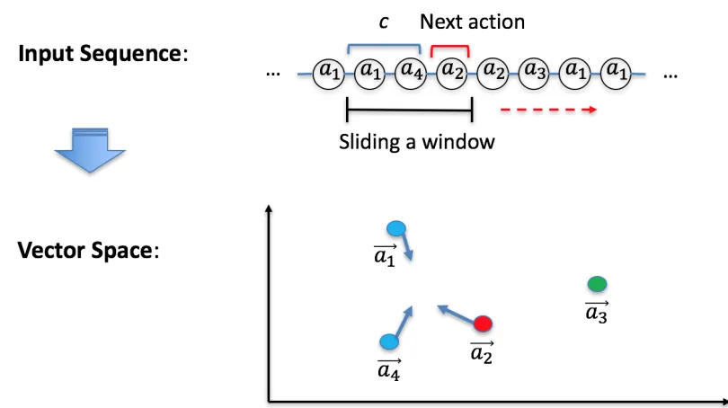
If some actions have frequently occurred close to each other in the sequence, our model ensure they become close to each other in the vector space. To train the vectors, we slide a window along with the input sequence as shown in Figure 2.3. The window contains the next action and the previous actions (i.e., contexts). We train the vector representations to ensure that the averaged vector of previous actions, which is denoted asvc, is close to the vector of the next action.
To predict the next action of a given context, our vector model extends CBOW by (1) modifying the Hierarchical Softmax function, (2) adding an additional output vector matrixW0
Figure 2.3Sliding a Window for the Vector Model
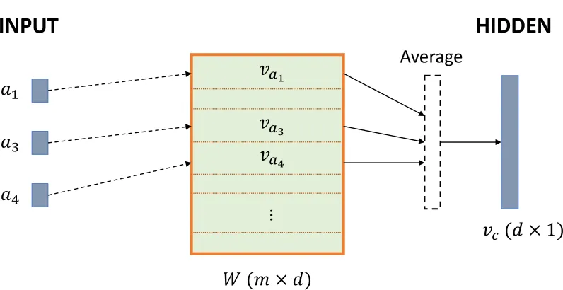
for the context vectorvc. We first explain how to make the vectorvc, then we describe Hierarchical Softmax and our modifications to it; finally, we outline how these are used to compute a score for actions. Figure 2.4 shows the input layer and hidden layer of a neural network with an example of an input sequence (a1,a3,a4). Firstly, from the input to the hidden layer, the vectorvc is generated. The vectorvc represents the set of input actions. Each node of the input layer indicates an action in the given recent sequence, and there is a matrixW between the Input and Hidden layers. Each row of this matrix consists of an input vector. In this case, the input vector ofa1is in the first row and
the input vector ofa3is in the third row. The vector model projects the vectorvc into the hidden layer by averaging all of these vectors of input actions.
2.4.2.1 Hierarchical Softmax
Computingψ(sn+1=ak|c)with the Softmax function (2.1) is expensive because we have to iterate through the vector representations of every word in the vocabulary. We use Hierarchical Soft-max[MB05]with the Huffman tree to reduce this complexity, as proposed by Mikolov et al.[Mik13b], and compute an approximate Huffman code of a target action.
INPUT
HIDDEN
!
"!
#!
$%
&() × 1)
…
- (. × ))
%
/0%
/1%
/2Average
1
Figure 2.4Vector Model between Input layer and Hidden layer
in the Huffman tree that encodesAs e e n(Equation 2.4), whereAs e e nare the actions that have been observed in the training dataset. We select the nodes for the set of inner-nodes by taking the nodes on the path starting at the root and ending atAs e e n. Letn(ak,j)represent the thejt hnode on the path from the root of the tree to the leaf node representing the target actionak. The Hierarchical Softmax defines the probability ofakbeing the next action given a contextc as follows:
n(a2,1)
n(a2,2)
n(a2,3)
a1 a2 a3 a4 a5 a6 a7 a8 0
0
1
ψ(sn+1=ak|c) =
L(ak)−1
Y
j=1
σ(¹·ºv 0
n(ak,j)
T
·vc) (2.4)
whereL(ak)is the length of the path,σ(z) = (1+e x p(−z))−1,¹·ºis¹n(ak,j+1) =c h(n(ak,j))º, c h(n(ak,j))is the left child of a noden(ak,j), andvn0(ak,j)is the vector of the inner noden(ak,j).
¹·ºbecomes 1 if a noden(ak,j+1)is the left child of the noden(ak,j)and−1 otherwise.
In the case of Figure 2.5, the probability ofa2being the next action given the contextc can be
computed as follows:
ψ(sn+1=a2|c) =σ(vn0(a2,1)
T
·vc)·σ(vn0(a2,2)
T
·vc)·σ(−vn0(a2,3)
T
·vc) (2.5)
where the path is from the rootn(a2, 1)to the leafa2, andL(a2) =4.
s
i#2%
s
i#1%
s
i%
W%
W%
W%
W’/W’
new%
Input%
Hidden%
Output%
v
c%
y"
Average%
Figure 2.6FVEC neural network architecture
2.4.2.2 Modified Hierarchical Softmax
turn left or right, we add a 0 or 1 to the code respectively. For example, in Figure 2.5,h(a2)is 001, because the path followed two left children, and terminated on a right child.
Therefore, to computey, we take the path from the root to the leaf node, and for each node on the path, we computeyj as follow:
yj =σ(−vn0(ak,j) T
·vc) (2.6)
where 1≤j≤lh(ak),σ(z) = (1+e x p(−z))
−1. This represents the probability of the code at position j,hj(ak), being 1.
2.4.2.3 Computing a Score for Actions
We consider two types of actions, computing heuristic scores separately for each. Firstly, we consider the actions,ak∈As e e n, that have occurred in the training dataset. Secondly, we consider the actions,
ak ∈An e w that are newly observed in the test or validation datasets and have never appeared in training dataset.
For an actionak∈As e e n, we compute the Huffman approximationydiscussed in Section 2.4.2.2. We then take the sum of squared errors betweenh(ak)andy(Equation 2.7) and compute the similarity by Equation (2.8).
For an actionak∈An e w, we first initialize an output vectorva0k if it is the first time thatak has
been observed.v0
ak is a column in the output vector matrixW
0
n e w. We then take the inner-product ofva0
k andvc and then convert it into a similarity score with the sigmoid function (Equation 2.9).
d(h(ak),y) = (h1−y1)2+...+ (hlh−ylh)
2 (2.7)
s i m(ak) =
1 1+d(h(ak),y)
, ifak∈As e e n (2.8)
s i m(ak) =
1 1+e x p(−vak0
T
·vc)
, ifak∈An e w (2.9)
s c o r e(ak) = lc
X
j=1
s i m(ak|sn−j+1, ...,sn) (2.10)
ψv e c(sn+1=ak|c) =
s c o r e(ak)
P
a∈A
s c o r e(a) (2.11)
2.4.3 Prediction
Finally, the normalized scores from these two models are combined to generate a final vote for all ak ∈A:
v o t e(sn+1=ak) =β·ψf r e q(sn+1=ak) + (1−β)·ψv e c(sn+1=ak) (2.12) where 0≤β≤1. Finally, the votes are ranked to find theN highest voted actions, which are used as our top-N predictions as shown in Figure 2.7.
1 Vector
Embedding Model
!"#$%(a1)
!"#$%(a2) . . !"#$%(am)
!&$'(a1)
!&$'(a2) . .
!&$'(am)
vote(a1) = ( ) !"#$%(a1) + (, − () )!&$'(a1) vote(a2) = ( ) !"#$%(a2) + (, − () )!&$'(a2) .
.
vote(am) = ( ) !"#$%(am) + (, − () )!&$'(am)
N highest scored actions Frequency Analysis Model
Figure 2.7Prediction
2.4.4 Updating the Vector Model
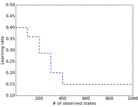
Figure 2.8Changes of The Learning Rateηt r a i n i n g
(c,ak), we also train the model with the contextsc0, the contexts of length less thanlc. For example, for the context/action pair((a1a2a3),a1), we train with((a3),a1),((a2a3),a1)and((a1a2a3),a1).
We set two different learning ratesηt r a i n i n g andηt e s t for the training and test sets respectively. During the training,ηt r a i n i n g is decreased toηt e s t linearly with the number of states that are seen so far in the sequence as shown in Figure 2.8. When updating the model during the test/validation phase, we fix the learning rate toηt e s t. We setηt r a i n i n g =0.4 andηt e s t =0.15 for our experiments over all datasets.
2.5
Empirical Evaluation
In this section, we first describe the datasets used for evaluation as well as the baseline methods. Then, we outline our parameter optimization process and, finally, discuss our experimental results.
2.5.1 Datasets
• UDC1- this dataset consists of logged behaviors from the Eclipse Integrated Development En-vironment (IDE) software tool. The data includes information on: loaded software bundles, commands accessed via keyboard shortcuts, actions invoked through menus (or toolbars), per-spective changes, usage of views, and usage of certain editor features. The dataset contains about 2.3 billion records from about 1.8 million unique users, captured from January 2009 to August 2010. We excluded records on software bundles in our training and test sets because they are not directly related to user actions. We identified the top 20 users with the most records and used only these records for our experiments - this reduced our evaluation dataset to 756, 130 records. • Word2- this dataset contains logs of user actions performed within the Microsoft Word application.
These logs include: copy, paste, and file open/save/print etc. The data represents 24 users and contains 74, 780 records covering two years from January 1997 to December 1998. Only the top 8 users with at least 2, 200 records each were used in our evaluation, reducing our dataset to 60, 312 records.
• Reality Mining3- this dataset consists of smart-phone usage data, including: call logs, user IDs, application usage, phone status (e.g., charging, idle, etc), user locations and so on[EP06]. It contains 95 users and spans September 2004 to June 2005. In our experiments, we extracted sequences of user ID, application usage and timestamp only. The top 84 users with at least 2, 200 records each were selected, providing 650, 756 records for our evaluation.
2.5.2 Baseline Methods
The prediction accuracy of FVEC was compared to four other sequential prediction methods, as well as a Null model.
• FxL[HS07]: This algorithm calculates a score for a possible next action by multiplying the Fre-quencyF of an action and the LengthLof the context. FxL builds upon an n-gram trie containing the frequencies of different input sub-sequences. The frequencies are weighted according to the lengths of the sub-sequences. FxL was chosen because it was the best performing algorithm among the existing prominent algorithms in[HS07]. We used our own implementation of this algorithm in Python.
• IPAM[DH98]: The Incremental Probabilistic Action Modeling method assumes that each action depends only on the previous action. It stores the probabilities of transitions from an action to a
1https://github.com/DeveloperLiberationFront/UsageDataCollectorOnBigData 2http://www.research.rutgers.edu/~sofmac/ml4um/
Figure 2.9Top-1,3 accuracy whenβ=0. Optimizing the value oflcusing UDC, Word and Reality Mining
validation datasets with 7900, 1900 and 1900 training respectively and 100 validation samples.
Figure 2.10Top-1,3 accuracy whenβ=1. Optimizing the value oflc using UDC, Word and Reality Mining
Figure 2.11Top-1 accuracy whenlc =5 for the frequency model andlc =2 for the vector model.
Opti-mizing the value ofβusing UDC, Word and Reality Mining validation datasets with 7900, 1900 and 1900
training respectively and 100 validation samples.
Figure 2.12Top-3 accuracy whenlc =5 for the frequency model andlc =2 for the vector model.
Opti-mizing the value ofβusing UDC, Word and Reality Mining validation datasets with 7900, 1900 and 1900
next action in ann+1 byntable, wherenis the number of actions (the(n+1)t hrow is called the defaultrow). The probabilities are updated by the use of an update function. A simple example of the update function is as follows: If an actionaj is seen following actionai, IPAM updates theit h row of the probability table by multiplying all elements of that row byαand increases element
(i,j)by(1−α), where 0≤α≤1. IPAM uses the same update function for thedefaultrow, but it is applied to thedefaultrow for every action seen. Thisdefaultrow is used to initialize rows for new actions. Again, we used our own implementation of this algorithm in Python.
• RNN[Elm90]: Recurrent Neural Networks are a class of neural network that exhibit temporal behavior as a result of feedback between units. This allows them to easily maintain states using an arbitrary number of previous inputs. Here, we use a form of partially recurrent neural network known as an Elman network. This network consists of three layers (input, hidden, and output), with the addition of ‘context units’, which take their input from hidden units. The number of context units and hidden units is the same. An advantage of Elman nets over other forms of RNN is that the number of context units is not determined by the output dimension but, instead, by the number of hidden units, which are easy to add and remove. For this implementation, we used the
RSNNS
R package.• HMM: In a Hidden Markov Model we assume our sequence data is a Markov process with hidden states. This makes the assumption that the next user-action depends only on the current hidden states of the model (which might correspond roughly to a user ‘task’ or ‘workflow’). We use a custom implementation in R of the well-known Baum-Welch algorithm to find the unknown parameters.
• Null: Our null model uses a simple heuristic for top-N prediction. To predict the next statesn+1
given a sequenceS= (s1,s2, ...,sn), we simply choose the most recently seen statesnas the top-1 prediction; for the top-2 prediction, we also includesn−1wheresn−16=sn, and so on until we have our top-N predictions.
2.5.3 Training, Validation and Test Sets
Figure 2.13Top-1 accuracy for UDC dataset with various test sizes
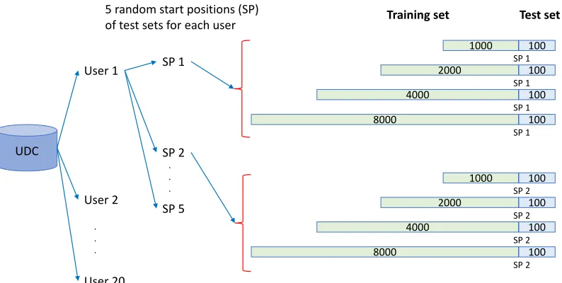
UDC User 1 . . . User 2 User 20
5 random start positions (SP) of test sets for each user
SP 1 SP 2 . . . SP 5 1000 100 SP 1 2000 100 SP 1 4000 100 SP 1 8000 100 SP 1
Training set Test set
1000 100 SP 2 2000 100 SP 2 4000 100 SP 2 8000 100 SP 2 1
Figure 2.15Creating Training and Test Sets
training set, we choose thensequential records for each user prior to the start of each test set, where 1000≤n≤8000 for the UDC dataset as shown in Figure 2.15, and 500≤n≤2000 for the Word dataset and the Reality Mining dataset. From thesenrecords, we use the last 100 records as our “validation set" to optimize the parameters of FVEC.
Table 2.2 shows the number of unique actions for each training size for each dataset. It shows the minimum, maximum and average number of actions in the training sets and the number of new actions in the test sets. The new action means that it has not appeared in the training set.
2.5.4 Selecting Parameters for FVEC
FVEC depends mainly on two parameters: the weighting parameterβand the context lengthlc. Figures 2.9 - 2.12 show the accuracy results of the top-1 and top-3 prediction on the validation set for a range of values for each parameter. The results shown use the largest value ofnfor each training set and are the average values of the five test sets over all users.
Figures 2.9 and 2.10 show that, whenβ=0 (i.e. only using the vector model), the accuracy is highest for smalllc. Whenβ=1 (i.e., only using the frequency model), the best results are obtained at approximatelylc =5. To maximize the accuracy for each model and for the combination of the two models, we selectlc =2 for the vector model andlc =5 for the frequency model.
Figure 2.16Top-1 standard deviation for UDC dataset with various test sizes
Table 2.2Number of Unique Actions
Dataset n Training New Actions in 100 Test Samples
UDC
Min Max Mean Min Max Mean
1000 12 79 47.17 0 5 1.24
2000 14 95 57.99 0 5 0.67
4000 14 113 69.71 0 4 0.41
8000 28 133 83.87 0 2 0.27
Word
Min Max Mean Min Max Mean
500 19 62 32.28 0 15 2.80
1000 28 80 45.38 0 10 1.58
1500 39 91 53.25 0 10 1.30
2000 42 97 60.10 0 9 1.15
RealityMining
Min Max Mean Min Max Mean
500 7 31 14.71 0 12 0.93
1000 8 37 18.39 0 10 0.65
1500 10 42 21.42 0 10 0.51
2000 10 51 24.82 0 9 0.42
2.5.5 Experimental Results
FVEC was compared against the baseline methods as well as CBOW, implemented in thegensim python package4, for top-1 and top-3 prediction accuracy on the three datasets. For the online algorithms (FVEC, IPAM and FxL), we built models from the training datasets and updated them at each state within the test datasets. Generating RNN and HMM models was found to be expensive at runtime, so it was unrealistic to rebuild their models every time a new data point was seen.
Tables 2.3, 2.4 and 2.5 show the experiment results for the UDC, Word and RealityMining datasets, respectively. The experimental results for top-1 and top-3 predictions were achieved using the following parameters: for FVEC, we usedd =30,β=0.4,lc=2 for the vector model andlc =5 for the frequency model; for FxL, we usedk=6 (meaning the context size is 5) as this achieved the best results in our experiments; and for IPAM, we useα=0.8 (as suggested in[DH98]). The parametern represents the training dataset size,|As e e n|is the number of unique actions (given as the mean over all training sets), and the results showing the highest accuracy are shown in bold.
Results for the vector model only (β=0) and for the frequency model only (β=1) are included in the tables. It can be seen that the FVEC ensemble (withβ=0.4) consistently outperforms all other
Figure 2.18FVEC and Each Model
methods for both top-1 and top-3 predictions. In addition, for some cases, only using the frequency portion of FVEC gives better results than the other methods.
Figure 2.18 shows the prediction accuracy of FVEC and each model according to the different Top-N predictions. Thex-axis indicates the numberN that indicates how many actions we determine for the prediction. They-axis indicates the prediction accuracy as a percentage. The red line denotes FVEC, the blue line is the Frequency model, and the black line is the Vector model. The Frequency model tends to give a higher accuracy than the vector model whenN is lower than 4. The Vector model tends to have a higher accuracy than the frequency model whenN is higher than 4. The ensemble of the score results from the two models produces a high accuracy for both low and high Top-N predictions.
In addition, we ran experiments on various test sizes to compare our method to other online algorithms (FxL and IPAM). Figures 2.13 - 2.17 show the accuracy and standard deviation results for the UDC dataset withn=8000 training set. FVEC shows consistently better accuracy and lower standard deviation than FxL and IPAM as the test size increases.
Figure 2.19Top-N accuracy for UDC dataset
Figure 2.21Top-N accuracy for Reality Mining dataset
Table 2.3Top 1 and 3 Prediction Accuracy over UDC dataset. All are % values exceptnand|As e e n|.
Top N n |As e e n| FVEC Vector Frequency FxL IPAM RNN HMM Null
(β=0.4) (β=0) (β=1)
Top 1
1000 47.2 48.61 41.50 47.85 48.22 46.57 38.33 19.72 34.80 2000 58.0 49.39 43.48 48.66 48.40 46.91 40.37 20.62 34.80 4000 69.7 50.38 44.56 49.71 48.63 46.96 42.95 21.10 34.80 8000 83.9 50.89 44.71 50.45 48.36 47.12 43.88 21.55 34.80
Top 3
1000 47.2 68.40 61.59 65.58 68.08 67.42 52.71 41.61 56.22 2000 58.0 70.59 64.71 68.36 69.27 67.87 56.25 41.85 56.22 4000 69.7 71.62 65.99 69.74 70.09 67.85 58.93 41.97 56.22 8000 83.9 72.54 67.58 71.07 70.37 67.86 60.80 41.67 56.22
Table 2.4Top 1 and 3 Prediction Accuracy over Word dataset. All are % values exceptnand|As e e n|.
Top N n |As e e n| FVEC Vector Frequency FxL IPAM RNN HMM Null
(β=0.4) (β=0) (β=1)
Top 1
500 32.3 48.28 40.15 47.72 47.75 47.07 39.82 20.37 28.02 1000 45.4 48.97 42.92 48.18 47.65 47.37 43.87 17.95 28.02 1500 53.3 49.58 45.02 48.38 48.15 47.42 45.25 20.35 28.02 2000 60.1 50.05 45.53 48.58 48.28 47.42 44.22 19.60 28.02
Top 3
500 32.3 68.75 63.58 65.85 68.20 67.02 60.25 47.37 57.05 1000 45.4 70.00 65.60 67.85 69.55 67.17 63.15 45.32 57.05 1500 53.3 70.35 66.95 68.30 68.77 67.07 63.30 47.07 57.05 2000 60.1 71.05 67.82 68.82 68.92 67.07 64.07 45.85 57.05
Table 2.5Top 1 and 3 Prediction Accuracy over Reality Mining dataset. All are % values exceptnand
|As e e n|.
Top N n |As e e n| FVEC Vector Frequency FxL IPAM RNN HMM Null
(β=0.4) (β=0) (β=1)
Top 1
500 14.2 53.33 48.28 52.49 52.19 50.85 50.24 45.31 24.25 1000 18.4 54.06 48.65 53.42 52.66 50.92 51.61 45.36 24.25 1500 21.4 54.29 49.00 53.92 52.71 50.95 51.76 45.19 24.25 2000 24.8 54.42 48.98 54.14 53.04 51.00 52.04 45.21 24.25
Top 3
500 14.2 82.30 78.79 79.89 81.07 81.21 78.54 75.17 76.76 1000 18.4 82.89 79.99 80.95 81.56 81.26 79.44 74.98 76.76 1500 21.4 83.19 80.45 81.40 81.83 81.29 79.78 74.88 76.76 2000 24.8 83.35 80.69 81.79 81.87 81.32 79.70 74.56 76.76
2.6
Summary
In this paper, we have proposed an ensemble prediction algorithm for user actions by combining a frequency model and a vector model. We show that this ensemble method has a higher prediction accuracy than both models in isolation. Moreover, from our online performance tests, FVEC always had a higher accuracy and a lower standard deviation than the other online sequential prediction algorithms.
CHAPTER
3
INFERRING MISSING ENTITIES AND
RELATION TYPES
3.1
Introduction
Knowledge Graphs (KGs) have recently become mainstream in IT companies, such as Google, Facebook, Microsoft, and Yahoo, as a way of storing information about entities and enhancing search results based on the captured semantic information. KGs store information as SPO triples, with each triple consisting of two entities (subject and object) and the relationship (predicate), for example (

![Figure 3.1 Sample Knowledge Graph. Figure adapted from [Nic16a].](https://thumb-us.123doks.com/thumbv2/123dok_us/1650278.1206628/52.612.169.462.106.222/figure-sample-knowledge-graph-figure-adapted-nic-a.webp)