Optimal Design Techniques for Distributed Parameter Systems
∗H.T. Banks
†D. Rubio
‡N. Saintier
§M.I. Troparevsky
¶Abstract
Parameter estimation problems consist in approximating parameter values of a given mathematical model based on measured data. They are usually formulated as optimization problems and the accuracy of their solutions depends not only on the chosen optimization scheme but also on the given data. The problem of collecting data in the “best way” in order to assure a statistically efficient estimate of the parameter is known asOptimal Design. In this work we consider the problem of finding optimal locations for source identification in the 3D unit sphere from data on its boundary. We apply three different optimal design criteria to this 3D problem: the Incremental Generalized Sensitivity Function (IGSF), the classicalD-optimal criterion and the SE-criterion recently introduced in [3]. The estimation of the parameters is then obtained by means of the Ordinary Least Square procedure. In order to analyze the performance of each strategy, the data are numerically simulated and the estimated values are compared with the values used for simulation.
1 Introduction.
In a series of recent works [1, 2, 3, 5, 6] several authors have developed a design framework based on the Fisher Information Matrix (FIM) for a system of differential equations to determine when and where an experimenter should take samples and what variables to measure in collecting information on a physical or biological process that is modeled by a vector dynamical system. This framework has also been proposed for use in inverse problem methodologies in the context of dynamical system or mathematical model parameter estimation when a sufficient number of observations of one or more states (variables) are available. Experimental design using the Fisher Information Matrix (FIM), which is based on sensitivity matrices (traditional and generalized), is described in [2] for the case of scalar data. In [3], the authors develop an experimental design theory using the FIM to identify optimal sampling times for experiments on physical processes (modeled by an ODE system) in which scalar or vector data will be taken. In addition to when and where to take
samples, the question ofwhat variables to measure is also very important in designing effective
experiments, especially when thenumber of state variables is large and this is discussed in [5, 6].
The methodology can be readily applied to problems involving ordinary, partial and delay
differential equations dynamics but requires both amathematical modeland astatistical model. In
particular one could consider a mathematical model in the form of a partial differential equation that is first order in time and second order in space
∂u
∂t = F(t, x, u, ∂u ∂x,
∂2u
∂x2, θ), t∈[t0, tf], x∈[x0, xf]
(1.1)
with appropriate boundary and initial conditions, whereu(t, x; ) is them-vector of state variables
of the system generated using a parameter vector θ ∈ Rp. A corresponding observation process
might be of form
(1.2) f(t, x;θ) =Cu(t, x;θ),
whereCis an observation operator that mapsRm→RN, whereN < mis the number of variables
observed at a single sampling time and location.
∗Supported by AFOSR Grants FA9550-10-1-0037 and FA9550-12-1-0188. †Center for Research in Scientific Computation, NCSU, USA.
‡Centro de Matem´atica Aplicada, UNSAM, BA, Argentina. §Instituto de Ciencias, UNGS, BA, Argentina.
In order to discuss uncertainty in parameter estimates, we may formulate a statistical model [16] of the form (this corresponds to an Ordinary Least Squares (OLS) fit to data formulation)
(1.3) Y(t, x) =f(t, x;θ0) +E(t, x), t∈[t0, tf], x∈[x0, xf],
where θ0 is the hypothesized true values of the unknown parameters and E is a vector random
process that represents observation error for the measured variables. Realizations of the statistical model (1.3) can be written
y(t, x) =f(t, x;θ0) +ǫ(t, x), t∈[t0, tf], x∈[x0, xf].
When collecting experimental data, it is often difficult to take continuous measurements of the
observed variables. Instead, we assume that we havekn observations at sampling points (ti, xj),
i= 1, . . . , k, j = 1, . . . , n, in periods [t0, tf]×[x0, xf]. We then write the observation process (1.2)
as
(1.4) f(ti, xj;θ) =Cu(ti, xj;θ), i= 1, . . . , k, j = 1, . . . , n,
the discrete statistical model as
(1.5) Yij =f(ti, xj;θ0) +E(ti, xj), i= 1, . . . , k, j= 1, . . . , n,
and a realization of the discrete statistical model as
yij =f(ti, xj;θ0) +ǫ(ti, xj), i= 1, . . . , k, j = 1, . . . , n.
Given a set of datayij, we could attempt to estimate θ0 in a process known as the inverse
problem. In previous efforts such an estimation framework has been successfully used with several models [5] including an experimentally validated six-compartment HIV model and a thirty-eight dimensional enzyme kinetics model of the Calvin Cycle in spinach. Here we illustrate ideas in
the context of estimation of the parameterθ of a stationary process modeled by a Poisson type
equation in 3D of the form
∆u(x) =g(x, θ) x∈G
(1.6)
whereθ∈Rp,Gis the unit ball ofR3,u(x)∈Ris the output andg:R3+p→Ris the source.
We suppose that there exists a real valueθ0such that the equation (1.6) describes the process.
The parameter valueθ0 is going to be estimated by an OLS procedure from values of the output
u(x) measured at a finite set of pointsx1, . . . , xn∈∂G. Given an initial set of observation points
Λ ={x1, ...,˜ x˜n} on∂G, an application of the OLS method yields an estimate ˆθΛ.
However different choices of the pointsx1, . . . , xn may lead to parameter estimates that could
be significantly different from a statistical point of view. In consequence it is important to look
for theoptimal set of observation pointsx1, . . . , xn, those that will lead to an accurate parameter
estimation. This is the purpose of the so-calledOptimal Designmethods (see [1], [2]).
In this work we numerically study the accuracy of the estimates ofθ in equation (1.6), based
on three optimal design criteria:
• maximizing the absolute value of the Incremental Generalized Sensitivity Function (IGSF),
introduced in [17];
• the well-knownD-optimal criterion (see [1], [2]);
• theSE-optimal design criterion, introduced in [3].
These three criteria give three different sets of observation points on∂G. Applying OLS we
then obtain three estimates ˆθGSF, ˆθD, ˆθSE of θ0.
2 Problem Formulation.
2.1 Mathematical model.As noted above we consider the Poisson equation with sourceg(x, θ) and Neumann boundary condition
∆u = g(x, θ) xin G,
(2.7)
∂u
∂ν = 0 xin∂G,
(2.8)
whereGis is the unit ball ofR3 . Existence, uniqueness of a solution uand its dependence with
respect to the parameters have been effectively studied (see [9, 10, 11, 13]). We associate the source to an electric dipole and represent it by
(2.9) g(x, θ) =∇ ·(qδ(x−rq)),
whereδis the Dirac distribution,rq = (rq1, rq2, rq3) is a fixed point inGandq= (q1, q2, q3)∈R3
is the dipole moment. This type of source appears in a number of real life problems. The
parameters of the model are thenθ= (rq, q)∈R6. We denote byu(x, θ) the solution of (2.7)-(2.9)
corresponding toθ.
2.2 Inverse problem.We assume that the value ofu|∂G, corresponding to the true parameter
θ0= (rq0, q0), has been measured atnpointsx1, .., xn ∈∂Gobtaining data of the form
u(x1, θ0) +ǫ1, ..., u(xn, θ0) +ǫn,
where ǫ1, .., ǫn are independent realization of a centered normal random variable with variance
σ2. The inverse problem consists in estimating the unknown parametersθ0 from these noisy data
ui:=u(xi, θ0) +ǫi,i= 1, .., n.
A well-known method to estimateθ0is to consider the ordinary least-square (OLS) functional
J(θ) =
n
X
i=1
(u(xi, θ)−ui)2.
The OLS-estimate ˆθ ofθ0 is defined as
ˆ
θ= argminθJ(θ).
Notice that ˆθis a realization of a random variable ˆΘ due to the presence of the random noise.
It can be proved that under suitable hypothesis, ˆΘ has asymptotically normal distribution (see
[4, 16])
(2.10) Θˆ ∼N(θ0,(F(x1, .., xn, θ0))−1),
whereF(x1, .., xn, θ) = (Fij(x1, .., xn, θ))i,j=1,..,6is the so-called Fisher information matrix defined
by
(2.11) Fij(x1, .., xn, θ) =σ−2
n
X
k=1 ∂u ∂θi
u(xk, θ)
∂u ∂θj
u(xk, θ).
We abuse notation and omit the dependence of all quantities and the numbernof points. A
precise discussion of the approximations involved in the above statements is given in [4].
3 Optimal design.
The optimal design problem consists in finding the points x1, .., xn in ∂G at which u is to be
measured, that will lead to an accurate estimation ofθ0. In view of the asymptotic distribution
(2.10)-(2.11) it is natural to choose the pointsxiin order to minimizeF(x1, .., xn, θ0) in some sense
(see [1], [2]).
• one based on the Incremental Generalized Sensitivity Function,
• the D-optimal criteria,
• the SE-optimal criteria.
3.1 Incremental Generalized Sensitivity Function.The Generalized Sensitivity Function was introduced by Thomaseth and Cobelli in [17] to analyze the information content in a data set with respect to the model parameters. It was meant to understand how the estimation of model parameters is related to observed system output. In that work, Thomaseth and Cobelli introduce the Generalized Sensitivity Functions along with the Incremental Generalized Sensitivity Functions. Their definitions were introduced for a dynamical system as discrete functions defined on a finite set of observations at some time instants. For the problem we are interested in, the observations
are taken at spatial pointsx1, ..., xn on∂Gand those functions are given by
(3.12) gs(xk) =σ−2
k
X
j=1
[F−1∂u(xj, θ0)
∂θ ]·
∂u(xj, θ0)
∂θ ,
fork= 1, ..., nwhere the symbol “·” in (3.12) represents element-by-element vector multiplication, and the Incremental Generalized Sensitivity Functions
(3.13) gsinc(xj) =gs(xj)−gs(xj−1),
that is,
(3.14) gsinc(xj) =σ−2F−1×
∂u(xj, θ)
∂θ ·
∂u(xj, θ)
∂θ ,
whereF =F(x1, .., xn, θ) is the Fisher information matrix defined in (2.11).
As it can be observed,gsdepends on the order of the points, hence it is not appropiate for our
problem. On the contrary,gsinc does not depend on the order of the points and it is suitable for
our purpose of finding ”best” observation points. In [17], the authors observed thatgsinc(xk) are
useful to quantify the information on parameters provided byu(xk). Based on this, we introduce
an optimal design method consisting in looking for then pointsx1, ..., xn in a large collection of
points where|gsinc|achieves its highest values.
3.2 D-optimal and SE-optimal.The so-called D-optimal design consists in minimizing detF(x1, ...xn, θ)−1. Geometrically, it corresponds to minimize the volume of the confidence
el-lipsoid for the covariance matrixF−1.
The SE-optimal design is another criterion recently introduced in [3] which turned out to be quite efficient. It consists in minimizing the standard errors namely
X
i
(F(x1, ...xn, θ)−1)ii.
4 Numerical results.
To test the relative merits of the proposed methods, we perform numerical experiments to study
the accurracy of the different estimates ˆθΛ, ˆθGSF, ˆθD, ˆθSE as follows. We first generate simulated
data
u(x1, θ0) +ǫ1, ..., u(xn, θ0) +ǫn,
where θ0 = (rq0, q0) with rq0 = (0.3,0.4,0), q0 = (3,4,0.1) and n is the number of observation
points. The perturbations ǫ1, .., ǫn are independent realizations of a centered normal random
An initial set Λn ={x1, ...,˜ x˜n}of observation points is taken on ∂Gas follows. We define a
mesh in the spherical coordinates (α, φ) with (α, φ)∈[0, π]×[0,2π] taking a uniform partition of
31 points inαand inφ, ordered as
(α1, φ1), ...,(α1, φ31), ...,(α31, φ1), ...,(α31, φ31).
We then obtain the meshMof 961 points on the surface∂Ggiven by
(4.15) M={xk= (sin(αi) cos(φj),sin(αi) sin(φj),cos(αi)), k= (i−1)∗31 +j}.
The initial set Λn={x1, ...,˜ x˜n} of observation points is chosen fromMtaking
(4.16) x˜i =xk, k= 100 + (i−1)
550
n−1, i= 1, ..., n.
As an initial guess for (rq0, q0) we consider
(4.17) θg= (rqg, qg),
with
(4.18) rqg= (0.2,0.5,0.1,), qg= (3.5,4.2,0.1).
The initial relative errors are
krq0−rqk
krq0k
= 0.35 kq0−qk
kq0k = 0.11.
We use four methods to estimateθ0:
• Method 1: An estimate ˆθΛ is obtained performing OLS with the initial guessθg defined in
(4.17) and the set Λn of observation points given by (4.16).
On the other hand, using the initial guessθg, three estimates ˆθGSF, ˆθD and ˆθSE of θ0 are
obtained applying OLS using the observation points arising from the three following optimal design criteria, respectively:
• Method 2: maximizing the absolute value of the Incremental Generalized Sensitivity
Function over the mesh M. That is, we compute IGSF on each point of M, using the
formulae given in (3.14),
gsinc(xk) =σ−2F−1×
∂u(xk, θg)
∂θ ·
∂u(xk, θg)
∂θ ,
for k=1,..,961. Then we pick the n points at which the absolute value of ISGF takes its
highest values. Therefore, we obtain a set ΛIGSF ofn”optimal” observation points that will
be used to perform OLS.
• Method 3: theD-optimal criterion. We look for a set ΛDofnobservation points minimizing
the function
detF(x1, ...xn, θg)−1
starting with Λn as initial guess points. We then perform OLS with ΛD and θg as initial
guess.
• Method 4: the SE-optimal design criterion. In this case, we look for a set ΛSE of n
observation points minimizing the function
X
i
(F−1
ii (x1, ...xn, θg)),
starting with Λn as initial guess points. We then perform OLS with ΛSE and θg as initial
guess.
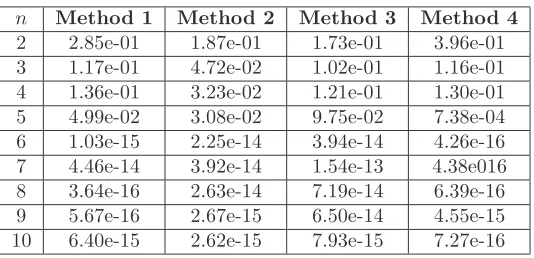
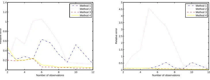
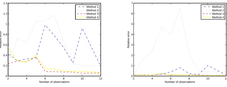
For each of these four estimates we calculate the standard errors and relative errors between
the estimated parameter ˆθ= ( ˆrq,qˆ) and the true valuesθ0= (rq0, q0).
The following tables and figures show the average of the relative errors and standard errors
2 2.85e-01 1.87e-01 1.73e-01 3.96e-01
3 1.17e-01 4.72e-02 1.02e-01 1.16e-01
4 1.36e-01 3.23e-02 1.21e-01 1.30e-01
5 4.99e-02 3.08e-02 9.75e-02 7.38e-04
6 1.03e-15 2.25e-14 3.94e-14 4.26e-16
7 4.46e-14 3.92e-14 1.54e-13 4.38e016
8 3.64e-16 2.63e-14 7.19e-14 6.39e-16
9 5.67e-16 2.67e-15 6.50e-14 4.55e-15
10 6.40e-15 2.62e-15 7.93e-15 7.27e-16
Table 1: Mean relative errors forrq whenσ= 0.
n Method 1 Method 2 Method 3 Method 4
2 1.02e-01 1.06e-01 1.10e-01 1.02e-01
3 1.04e-01 1.04e-01 1.05e-01 1.04e-01
4 1.03e-01 7.66e-02 1.02e-01 1.02e-01
5 1.58e-02 7.32e-02 3.34e-02 2.25e-04
6 4.94e-16 4.59e-14 1.38e-13 3.45e-16
7 3.30e-14 7.98e-14 2.32e-13 4.83e-16
8 1.96e-16 4.42e-14 5.05e-14 4.20e-16
9 2.28e-16 6.88e-15 2.21e-13 1.43e-15
10 2.95e-15 5.78e-15 7.01e-15 1.50e-16
Table 2: Mean relative errors forqwhenσ= 0.
2 4 6 8 10 12 0
0.05 0.1 0.15 0.2 0.25 0.3 0.35 0.4
Number of observations
Relative error
Method 1 Method 2 Method 3 Method 4
2 4 6 8 10 12 0
0.02 0.04 0.06 0.08 0.1 0.12
Number of observations
Relative error
Method 1 Method 2 Method 3 Method 4
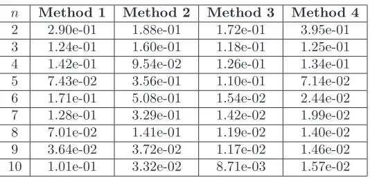
n Method 1 Method 2 Method 3 Method 4
2 2.90e-01 1.88e-01 1.72e-01 3.95e-01
3 1.24e-01 1.60e-01 1.18e-01 1.25e-01
4 1.42e-01 9.54e-02 1.26e-01 1.34e-01
5 7.43e-02 3.56e-01 1.10e-01 7.14e-02
6 1.71e-01 5.08e-01 1.54e-02 2.44e-02
7 1.28e-01 3.29e-01 1.42e-02 1.99e-02
8 7.01e-02 1.41e-01 1.19e-02 1.40e-02
9 3.64e-02 3.72e-02 1.17e-02 1.46e-02
10 1.01e-01 3.32e-02 8.71e-03 1.57e-02
Table 3: Mean relative errors forrq whenσ= 0.05.
n Method 1 Method 2 Method 3 Method 4
2 1.02e-01 1.06e-01 1.10e-01 1.02e-01
3 1.04e-01 1.075e-01 1.05e-01 1.04e-01
4 1.03e-01 1.56e-01 1.03e-01 1.03e-01
5 3.32e-02 9.69e-01 4.32e-02 3.00e-02
6 6.74e-02 1.45e+00 2.09e-02 1.44e-02
7 1.19e-01 7.70e-01 1.73e-02 1.51e-02
8 3.04e-02 3.08e-01 1.72e-02 1.35e-02
9 2.15e-02 7.80e-02 1.63e-02 1.17e-02
10 9.23e-02 6.69e-02 1.20e-02 1.13e-02
Table 4: Mean relative errors forqwhen σ= 0.05.
2 4 6 8 10 12 0
0.1 0.2 0.3 0.4 0.5 0.6 0.7
Number of observations
Relative error
Method 1 Method 2 Method 3 Method 4
2 4 6 8 10 12 0
0.5 1 1.5
Number of observations
Relative error
Method 1 Method 2 Method 3 Method 4
2 3.09e-01 1.92e-01 1.81e-01 4.14e-01
3 1.49e-01 3.41e-01 1.41e-01 1.49e-01
4 1.58e-01 2.66e-01 1.45e-01 1.51e-01
5 1.21e-01 7.43e-01 1.37e-01 1.31e-01
6 3.47e-01 8.93e-01 3.00e-02 5.43e-02
7 2.50e-01 7.62e-01 2.77e-02 4.05e-02
8 1.59e-01 3.76e-01 2.23e-02 2.47e-02
9 8.35e-02 7.64e-02 2.38e-02 2.89e-02
10 2.16e-01 7.18e-02 1.66e-02 3.39e-02
Table 5: Mean relative errors forrq whenσ= 0.1.
n Method 1 Method 2 Method 3 Method 4
2 1.03e-01 1.06e-01 1.10e-01 1.03e-01
3 1.04e-01 2.42e-01 1.05e-01 1.04e-01
4 1.05e-01 4.68e-01 1.04e-01 1.04e-01
5 5.95e-02 2.69e+00 6.25e-02 5.87e-02
6 1.34e-01 2.89e+00 3.89e-02 3.46e-02
7 2.41e-01 2.53e+00 3.27e-02 2.80e-02
8 6.60e-00 1.00e+00 3.26e-02 2.52e-02
9 4.52e-02 1.64e-01 3.38e-02 2.36e-02
10 1.96e-01 1.49e-01 2.32e-02 2.27e-02
Table 6: Mean relative errors forqwhenσ= 0.1.
2 4 6 8 10 12 0
0.1 0.2 0.3 0.4 0.5 0.6 0.7 0.8 0.9
Number of observations
Relative error
Method 1 Method 2 Method 3 Method 4
2 4 6 8 10 12 0
0.5 1 1.5 2 2.5 3
Number of observations
Relative error
Method 1 Method 2 Method 3 Method 4
n Method 1 Method 2 Method 3 Method 4
2 3.38e-01 2.00e-01 1.98e-01 4.56e-01
3 1.91e-01 5.19e-01 1.77e-01 1.86e-01
4 1.92e-01 4.28e-01 1.66e-01 1.69e-01
5 1.79e-01 8.88e-01 1.77e-01 1.79e-01
6 5.33e-01 9.85e-01 4.41e-02 7.77e-02
7 3.87e-01 1.36e+00 4.28e-02 6.26e-02
8 2.32e-01 4.80e-01 3.47e-02 4.03e-02
9 1.13e-01 1.07e-01 3.55e-02 4.19e-02
10 3.62e-01 9.65e-02 2.65e-02 4.84e-02
Table 7: Mean relative errors forrq whenσ= 0.15.
n Method 1 Method 2 Method 3 Method 4
2 1.03e-01 1.06e001 1.10e-01 1.03e-01
3 1.05e-01 6.49e-01 1.05e-01 1.04e-01
4 1.07e-01 1.05e+00 1.07e-01 1.08e-01
5 8.73e-02 3.77e+00 8.09e-02 8.61e-02
6 2.13e-01 3.38e+00 5.89e-02 4.89e-02
7 3.54e-01 9.09e+00 4.99e-02 4.23e-02
8 1.00e-01 1.37e+00 5.22e-02 4.11e-02
9 6.83e-02 2.27e-01 5.17e-02 3.38e-02
10 3.58e-01 1.91e-01 3.51e-02 3.33e-02
Table 8: Mean relative errors forqwhen σ= 0.15.
2 4 6 8 10 12 0
0.2 0.4 0.6 0.8 1 1.2 1.4
Number of observations
Relative error
Method 1 Method 2 Method 3 Method 4
2 4 6 8 10 12 0
1 2 3 4 5 6 7 8 9 10
Number of observations
Relative error
Method 1 Method 2 Method 3 Method 4
2 3.68e-01 2.04e-01 2.00e-01 4.62e-01
3 2.19e-01 6.70e-01 1.86e-01 1.95e-01
4 2.75e-01 5.33e-01 2.00e-01 2.03e-01
5 2.28e-01 1.01e+00 2.33e-01 2.42e-01
6 6.34e-01 1.05e+00 5.99e-02 1.00e-01
7 5.60e-01 8.28e-01 5.87e-02 8.61e-02
8 3.23e-01 5.65e-01 4.43e-02 5.65e-02
9 1.59e-01 1.55e-01 4.84e-02 5.60e-02
10 5.20e-01 1.39e-01 3.34e-02 6.06e-02
Table 9: Mean relative errors forrq whenσ= 0.2.
n Method 1 Method 2 Method 3 Method 4
2 1.03e-01 1.06e-01 1.10e-01 1.03e-01
3 1.05e-01 1.00e+00 1.05e-01 1.04e-01
4 1.10e-01 1.49e+00 1.08e-01 1.09e-01
5 1.06e-01 4.58e+00 1.08e-01 1.20e-01
6 2.54e-01 3.84e+00 8.21e-02 6.21e-02
7 5.48e-01 3.22e+00 7.67e-02 6.61e-02
8 1.36e-01 1.80e+00 6.51e-02 5.41e-02
9 8.82e-02 3.47e-01 6.58e-02 4.86e-02
10 5.45e-01 2.92e-01 4.77e-02 4.58e-02
Table 10: Mean relative errors forqwhenσ= 0.2.
2 4 6 8 10 12 0
0.2 0.4 0.6 0.8 1 1.2 1.4
Number of observations
Relative error
Method 1 Method 2 Method 3 Method 4
2 4 6 8 10 12 0
0.5 1 1.5 2 2.5 3 3.5 4 4.5 5
Number of observations
Relative error
Method 1 Method 2 Method 3 Method 4
n Method 1 Method 2 Method 3 Method 4
2 4.35e-01 2.23e-01 2.37e-001 5.50e-01
3 2.89e-01 7.20e-01 2.86e-001 2.93e-01
4 3.29e-01 6.41e-01 2.72e-001 2.70e-01
5 3.42e-01 1.04e+00 3.65e-001 3.98e-01
6 9.81e-01 1.06e+00 8.66e-002 1.48e-01
7 7.76e-01 1.17e+00 8.28e-002 1.31e-01
8 5.45e-01 6.61e-01 7.60e-002 9.52e-02
9 2.55e-01 2.39e-01 7.65e-002 8.59e-02
10 9.20e-01 2.07e-01 5.22e-002 8.89e-02
Table 11: Mean relative errors forrq whenσ= 0.3.
n Method 1 Method 2 Method 3 Method 4
2 1.06e-01 1.06e-01 1.10e-01 1.08e-01
3 1.07e-01 1.66e+00 1.07e-01 1.07e-01
4 1.19e-01 2.36e+00 1.18e-01 1.19e-01
5 1.67e-01 4.68e+00 1.83e-01 2.45e-01
6 4.01e-01 3.96e+00 1.16e-01 9.30e-02
7 7.99e-01 6.51e+00 9.83e-02 1.03e-01
8 2.28e-01 2.12e+00 1.10e-01 8.96e-02
9 1.34e-01 5.22e-01 1.05e-01 7.41e-02
10 1.01e+00 4.11e-01 6.78e-02 6.07e-02
Table 12: Mean relative errors forqwhenσ= 0.3.
2 4 6 8 10 12 0
0.2 0.4 0.6 0.8 1 1.2 1.4
Number of observations
Relative error
Method 1 Method 2 Method 3 Method 4
2 4 6 8 10 12 0
1 2 3 4 5 6 7
Number of observations
Relative error
Method 1 Method 2 Method 3 Method 4
2 5.66e-01 2.54e-01 2.72e-01 5.6824e-001
3 4.15e-01 8.00e-01 3.74e-01 3.78e-01
4 5.08e-01 7.42e-01 3.72e-01 3.61e-01
5 5.04e-01 1.17e+00 4.85e-01 5.35e-01
6 1.01e+00 1.15e+00 1.25e-01 2.81e-01
7 1.03e+00 1.30e+00 1.08e-01 1.53e-01
8 1.21e+00 8.22e-01 9.35e-02 1.09e-01
9 3.48e-01 4.16e-01 9.55e-02 1.21e-01
10 1.13e+00 3.36e-01 7.21e-02 1.34e-01
Table 13: Mean relative errors forrq whenσ= 0.4.
n Method 1 Method 2 Method 3 Method 4
2 1.14e-01 1.06e-01 1.12e-01 1.11e-01
3 1.16e-01 2.65e+00 1.11e-01 1.12e-01
4 1.49e-01 3.42e+00 1.28e-01 1.28e-01
5 2.93e-01 5.96e+00 2.78e-01 3.57e-01
6 4.55e-01 4.26e+00 1.77e-01 1.77e-01
7 1.03e+00 9.90e+00 1.33e-01 1.22e-01
8 9.28e-01 3.16e+00 1.34e-01 9.80e-02
9 1.84e-01 1.19e+00 1.37e-01 9.68e-02
10 1.32e+00 7.49e-01 9.18e-02 9.50e-02
Table 14: Mean relative errors forqwhenσ= 0.4.
2 4 6 8 10 12 0
0.2 0.4 0.6 0.8 1 1.2 1.4
Number of observations
Relative error
Method 1 Method 2 Method 3 Method 4
2 4 6 8 10 12 0
1 2 3 4 5 6 7 8 9 10
Number of observations
Relative error
Method 1 Method 2 Method 3 Method 4
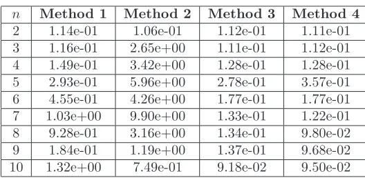
n Method 1 Method 2 Method 3 Method 4
2 6.60e-01 2.90e-01 3.26e-01 6.97e-01
3 4.91e-01 9.29e-01 4.62e-01 4.62e-01
4 5.83e-01 8.81e-01 5.27e-01 5.090e-01
5 5.97e-01 1.30e+00 5.90e-01 6.87e-01
6 1.40e+00 1.20e+00 1.65e-01 3.16e-01
7 1.37e+00 1.31e+00 1.61e-01 2.38e-01
8 1.10e+00 9.33e-01 1.20e-01 1.20e-01
9 4.04e-01 4.90e-01 1.15e-01 1.43e-01
10 1.51e+00 4.05e-01 7.90e-02 1.49e-01
Table 15: Mean relative errors forrq whenσ= 0.5.
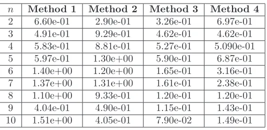
n Method 1 Method 2 Method 3 Method 4
2 1.24e-01 1.06e-01 1.12e-01 1.27e-01
3 1.26e-01 3.68e+00 1.20e-01 1.21e-01
4 2.05e-01 4.65e+00 1.77e-01 1.80e-01
5 3.76e-01 7.59e+00 3.65e-01 5.25e-01
6 6.65e-01 4.75e+00 2.28e-01 2.35e-01
7 1.87e+00 7.19e+00 1.87e-01 1.77e-01
8 6.33e-01 3.99e+00 1.77e-01 1.24e-01
9 2.14e-01 1.46e+00 1.63e-01 1.13e-01
10 2.35e+00 9.56e-01 1.13e-01 1.11e-01
Table 16: Mean relative errors forqwhenσ= 0.5.
2 4 6 8 10 12 0
0.2 0.4 0.6 0.8 1 1.2 1.4 1.6
Number of observations
Relative error
Method 1 Method 2 Method 3 Method 4
2 4 6 8 10 12 0
1 2 3 4 5 6 7 8
Number of observations
Relative error
Method 1 Method 2 Method 3 Method 4
2 3 4 5 6 7 8 9 10 11 12 0 0.1 0.2 0.3 0.4 0.5 0 0.2 0.4 0.6 0.8 1 1.2 1.4 1.6
Number of observations Noise
2 3 4 5 6 7 8 9 10 11 12
0 0.1 0.2 0.3 0.4 0.5 0 0.5 1 1.5 2 2.5
Number of observations Noise
Figure 9: Relative errors forMethod 1as a function of the number of observationsn and noise
σ.
2 3 4 5 6 7 8 9 10 11 12
0 0.1 0.2 0.3 0.4 0.5 0 0.2 0.4 0.6 0.8 1 1.2 1.4
Relative error for rq using Method 2
Number of observations Noise
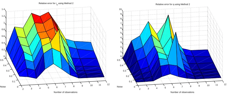
2 3 4 5 6 7 8 9 10 11 12
0 0.1 0.2 0.3 0.4 0.5 0 1 2 3 4 5 6 7 8 9 10
Relative error for q using Method 2
Number of observations Noise
Figure 10: Relative errors forMethod 2as a function of the number of observationsnand noise
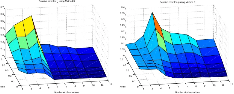
2 3 4 5 6 7 8 9 10 11 12 0 0.1 0.2 0.3 0.4 0.5 0 0.1 0.2 0.3 0.4 0.5 0.6 0.7
Relative error for rq using Method 3
Number of observations Noise
2 3 4 5 6 7 8 9 10 11 12
0 0.1 0.2 0.3 0.4 0.5 0 0.05 0.1 0.15 0.2 0.25 0.3 0.35 0.4
Relative error for q using Method 3
Number of observations Noise
Figure 11: Relative errors forMethod 3as a function of the number of observationsnand noise
σ.
2 3 4 5 6 7 8 9 10 11 12
0 0.1 0.2 0.3 0.4 0.5 0 0.1 0.2 0.3 0.4 0.5 0.6 0.7
Relative error for rq using Method 4
Number of observations Noise
2 3 4 5 6 7 8 9 10 11 12
0 0.1 0.2 0.3 0.4 0.5 0 0.1 0.2 0.3 0.4 0.5 0.6 0.7
Relative error for q using Method 4
Number of observations Noise
Figure 12: Relative errors forMethod 4as a function of the number of observationsnand noise
Method ( q(1)) ( q(2)) ( q(3))
6 Method 1 4.08e+02 5.30e+01 4.51e+02
Method 2 5.60e+03 5.95e+03 4.46e+03
Method 3 1.24e-02 9.12e-03 7.03e-03
Method 4 8.27e-03 1.58e-02 2.46e-02
8 Method 1 3.83e-02 3.14e-02 6.06e-02
Method 2 1.69e-01 1.24e-01 6.47e-02
Method 3 8.29e-03 6.30e-03 7.10e-03
Method 4 1.08e-02 6.39e-03 8.29e-03
10 Method 1 2.97e-02 1.21e-01 4.28e-02
Method 2 1.85e-02 1.82e-02 2.65e-02
Method 3 4.71e-03 4.53e-03 6.96e-03
Method 4 7.84e-03 1.25e-02 1.12e-02
Table 17: Mean standard error for each components ofrq = (rq(1), rq(2), rq(3)) withσ= 0.1.
n Method SE(q(1)) SE(q(2)) SE(q(3))
6 Method 1 4.72e+02 1.79e+03 1.57e+03
Method 2 3.74e+05 3.39e+05 1.46e+05
Method 3 1.49e-01 1.20e-01 1.28e-01
Method 4 9.62e-02 6.75e-02 1.31e-01
8 Method 1 1.66e-01 2.30e-01 1.82e-01
Method 2 3.79e+00 4.99e+00 1.46e+00
Method 3 1.28e-01 7.66e-02 1.07e-01
Method 4 1.05e-01 6.79e-02 7.89e-02 10 Method 1 9.23e-01 6.15e-01 5.03e-01
Method 2 4.62e-01 2.55e-01 5.41e-01
Method 3 6.46e-02 6.46e-02 9.17e-02
Method 4 7.48e-02 6.13e-02 7.23e-02
n Method SE(rq(1)) SE(rq(2)) SE(rq(3))
6 Method 1 8.01e002 1.29e+02 9.06e+02
Method 2 2.07e+04 7.13e+03 3.94e+03
Method 3 2.54e-02 1.84e-02 1.40e-02
Method 4 1.71e-02 3.21e-02 4.98e-02
8 Method 1 7.90e-02 6.33e-02 1.32e-01
Method 2 3.38e-01 3.01e-01 1.30e-01
Method 3 1.66e-02 1.26e-02 1.42e-02
Method 4 2.19e-02 1.27e-02 1.65e-02
10 Method 1 3.02e-01 6.09e-01 1.01e-01
Method 2 3.80e-02 3.78e-02 5.55e-02
Method 3 9.42e-03 9.07e-03 1.39e-02
Method 4 1.60e-02 2.52e-02 2.24e-02
Table 19: Mean standard error for each components ofrq = (rq(1), rq(2), rq(3)) withσ= 0.2.
n Method SE(q(1)) SE(q(2)) SE(q(3))
6 Method 1 1.52e+03 3.37e+03 3.32e+03
Method 2 3.71e+05 1.22e+05 1.95e+05
Method 3 3.05e-01 2.44e-01 2.58e-01
Method 4 1.91e-01 1.43e-01 2.66e-01
8 Method 1 3.83e-01 4.80e-01 3.99e-01
Method 2 8.42e+00 1.24e+01 3.57e+00
Method 3 2.58e-01 1.53e-01 2.14e-01
Method 4 2.12e-01 1.36e-01 1.58e-01 10 Method 1 7.84e+00 1.58e+00 4.85e+00
Method 2 9.88e-01 5.67e-01 1.15e+00
Method 3 1.29e-01 1.29e-01 1.83e-01
Method 4 1.50e-01 1.23e-01 1.44e-01
Method ( q(1)) ( q(2)) ( q(3))
6 Method 1 1.17e+05 2.16e+04 1.31e+05
Method 2 2.21e+04 1.37e+04 1.07e+04
Method 3 4.00e-02 2.81e-02 2.14e-02
Method 4 3.12e-02 5.28e-02 8.78e-02
8 Method 1 1.86e-01 1.12e-01 2.93e-01
Method 2 4.68e-01 4.07e-01 3.23e-01
Method 3 2.52e-02 1.92e-02 2.16e-02
Method 4 3.30e-02 1.95e-02 2.53e-02
10 Method 1 2.66e+00 7.99e+00 4.99e-01
Method 2 6.13e-02 5.53e-02 8.18e-02
Method 3 1.41e-02 1.36e-02 2.09e-02
Method 4 2.46e-02 3.79e-02 3.37e-02
Table 21: Mean standard error for each components ofrq = (rq(1), rq(2), rq(3)) withσ= 0.3.
n Method SE(q(1)) SE(q(2)) SE(q(3))
6 Method 1 2.05e+05 4.01e+05 5.19e+05
Method 2 8.62e+05 6.06e+05 3.72e+05
Method 3 4.74e-01 3.78e-01 3.91e-01
Method 4 3.05e-01 3.51e-01 4.43e-01
8 Method 1 6.21e-01 1.23e+00 8.32e-01
Method 2 1.94e+01 2.34e+01 6.35e+00
Method 3 3.90e-01 2.32e-01 3.26e-01
Method 4 3.15e-01 2.04e-01 2.39e-01 10 Method 1 1.30e+02 4.93e+01 5.00e+01
Method 2 1.47e+00 9.28e-01 1.75e+00
Method 3 1.94e-01 1.94e-01 2.75e-01
Method 4 2.26e-01 1.87e-01 2.17e-01
5 Example: The EEG Inverse Problem
The electric process underlying the generation of the electroencephalography (EEG) signals can be modeled as a set of current sources within the brain. Considering the velocity of propagation of the electric waves in the brain, the static approximation of Maxwell’s equations can be used to describe this process (see, e.g, [9], [12]). The resulting model is a 3D Poisson-type equation with interfaces
that relates the electric potentialuin the head with the impressed currentJi,∇ ·(σ∇u)) =∇ ·Ji.
The impressed curent is often represented by an electric dipole, i.e.,Ji(x) =qδ(x−rq), whereδis
the Dirac distribution,rq is the dipole location, andqis the dipole moment. The inverse problem
of EEG consists in findingrq andqfrom given scalp data u. This problem has been largely studied
and gave rise to a large amount of publications (see, e.g. [8], [9],[14],[15],[18],[19],[20] and references
therein). Since in practice the scalp potentialuis measured at a finite set of points in the scalp
(where the electrodes are placed) it is important to determine the location of the electrodes that
will lead to the best possible estimation ofrq andq.
If we consider a simplified model for the head: a spherical volume with constant conductivity, the parameter identification developed in this work for the Poisson equation (2.7) in the unit ball in
R3, can be seen as a solution to the inverse problem in EEG for this simplified model. We are
currently considering parameter estimation in more realistic multi-layer head models in the context of these optimal design techniques.
6 Conclusions
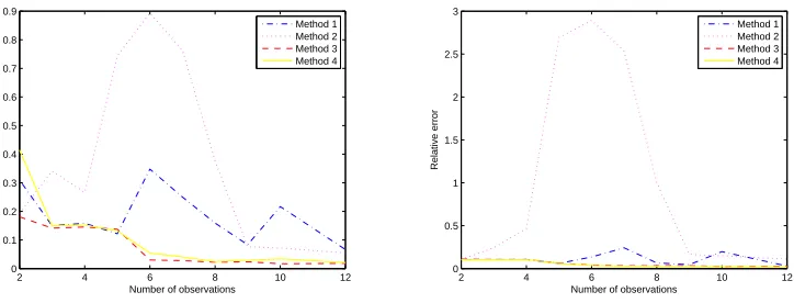
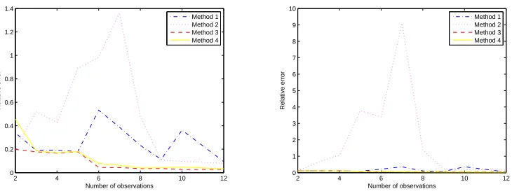
In summary, we are able to draw a number of conclusions from our results reported above.
• For noise free data, all methods are comparable. Forn= 5 the SE optimal makes a difference
whereas forn= 6 all methods produce good behavior.
• In all cases, relative errors are smaller for Methods 3 and 4. The difference increases as the
variance of the noise increases. Also, the difference is larger forn= 6 observations or more.
• Regarding standard errors, forn= 6 Methods 3 and 4 provide good results while the others
do not.
• For both measures (relative errors or standard errors), one can obtain good results when
n= 6. It appears to be of level value to consider more than 6 observations.
• In general methods 3 and 4 perform better and they provide comparable behavior.
In conclusion we believe optimal design is useful when the number of observations that can be collected is similar to the number of parameter values to be estimated. When many observations can be taken, even OLS without optimal design will work well, although it appears that applying optimal design techniques will yield more accurate estimates in any case.
References
[1] H. T. Banks, S. Dediu, and S. L. Ernstberger,Sensitivity functions and their uses in inverse problems, J. Inverse and Ill-posed Problems, 15 (2007), pp. 683–708.
[2] H. T. Banks, S. Dediu, S. L. Ernstberger and F. Kappel,A new optimal approach to optimal design
problem, J. inverse and ill-posed problems, 18 (2010), pp. 25–83.
[3] H. T. Banks, K. Holm, and F. Kappel,Comparison of optimal design methods in inverse problems, Inverse Probl., 1; 27 (7) (2011), pii: 075002.
[4] H. T. Banks, S. Hu, and W. C. Thompson, Modeling and Inverse Problems in the Presence of
Uncertainty, CRC Press, Boca Raton, FL., to appear.
[5] H.T. Banks and K.L. Rehm, Experimental design for vector output systems, CRSC-TR12-11, N. C. State University, Raleigh, NC, April, 2012.
[6] H.T. Banks and K.L. Rehm, Experimental design for distributed parameter vector systems CRSC-TR12-17, N. C. State University, Raleigh, NC, August, 2012;Applied Mathematics Letters,26(2013), 10–14; http://dx.doi.org/10.1016/j.aml.2012.08.003.
[7] J. A. Burns, D. Rubio, and M. I. Troparevsky, Sensitivity analysis for an Inverse Problem in
Bioengineering, ICNPAA, Mathematical Problems in Engineering and Aerospace Sciences, Budapest
MEG/EEG data contaminated with spatially and temporal correlated background noise, IEEE Trans. On Signal Processing, 50; 7 (2002), pp. 1565–1572.
[9] A. El Badia and T. Ha-Duong, An inverse source problem in potential analysis, Inverse Problems, 16, 3 (2000), pp. 651–663.
[10] L. C. Evans,Partial Differential Equations, Graduate Studies in Mathematics, American Mathemat-ical Soc., 1997.
[11] G. Folland,Introduction to Partial Differential Equations, Princeton University Press, Princeton, NJ, 1995.
[12] M. R. Hamalainen, R. J. Hari, J. Ilmoniemi, J. Knuutila, and O. Lounasmaa,
Magnetoencephalog-raphy, theory, instrumentation and applications to noninvasive studies of the working human brain,
Reviews of Modern Physics, 65 (1993), pp. 414–487.
[13] V. Isakov,Inverse Source Problems, Mathematical Surveys and Mongraphs, American Mathematical Soc., 1990.
[14] D. Rubio and M. I. Troparevsky,The EEG forward problem: theoretical and numerical aspects, Latin American Applied Research, 36 (2006), pp. 87–92.
[15] , Sensitivity analysis on a simplified model of the EEG inverse problem, Mec´anica
Computa-cional, 26 (2007), pp. 2086–2092.
[16] G. A. F. Seber and C. J. Wild,Nonlinear Regression, Wiley Intersciences, Hoboken, NJ, 2003. [17] K. Thomaseth and C. Cobelli,Generalized sensitivity functions in physiological system identification,
Annals of Biomedical Engineering, 27 (1999), pp. 607–616.
[18] M. I. Troparevsky and D Rubio,On the weak solutions of the forward problem in EEG, Journal of Applied Mathematics, 12 (2003), pp. 647–656.
[19] , Weak solutions of the forward problem in EEG for different conductivity values, Journal of
Mathematical and Computer Modeling, 41, 13, ( 2005), pp. 1403–1492.