Joint Mapping of Quantitative Trait Loci for Multiple Binary Characters

©

DOI: 10.1534/genetics.103.019406

Joint Mapping of Quantitative Trait Loci for Multiple Binary Characters

Chenwu Xu,* Zhikang Li

†

_{and Shizhong Xu*}

,1

*Department of Botany and Plant Sciences, University of California, Riverside, California 92521 and

†_{Chinese Academy of Agricultural Sciences, Beijing 100081, China}

Manuscript received June 26, 2003 Accepted for publication October 11, 2004

ABSTRACT

Joint mapping for multiple quantitative traits has shed new light on genetic mapping by pinpointing pleiotropic effects and close linkage. Joint mapping also can improve statistical power of QTL detection. However, such a joint mapping procedure has not been available for discrete traits. Most disease resistance traits are measured as one or more discrete characters. These discrete characters are often correlated. Joint mapping for multiple binary disease traits may provide an opportunity to explore pleiotropic effects and increase the statistical power of detecting disease loci. We develop a maximum-likelihood method for mapping multiple binary traits. We postulate a set of multivariate normal disease liabilities, each contributing to the phenotypic variance of one disease trait. The underlying liabilities are linked to the binary phenotypes through some underlying thresholds. The new method actually maps loci for the variation of multivariate normal liabilities. As a result, we are able to take advantage of existing methods of joint mapping for quantitative traits. We treat the multivariate liabilities as missing values so that an expectation-maximization (EM) algorithm can be applied here. We also extend the method to joint mapping for both discrete and continuous traits. Efficiency of the method is demonstrated using simulated data. We also apply the new method to a set of real data and detect several loci responsible for blast resistance in rice.

M

ULTIPLE traits are measured virtually in all line- true multivariate analysis in which a multivariate normal crossing experiments of QTL mapping. Yet, al- distribution is assumed for the multiple traits, and thus most all data collected for multiple traits are analyzed a multivariate Gaussian model is applied to construct separately for different traits. Joint analysis for multiple the likelihood function. Parameter estimation is con-traits has shed new light in QTL mapping by improving ducted via either the expectation-maximization (EM) the statistical power of QTL detection and increasing algorithm (Dempsteret al. 1977) or the multiple-traits the accuracy of QTL localization when different traits least-squares method (Knott and Haley2000). One segregating in the mapping population are genetically _{problem with these multivariate analyses is that if the} related. Joint analysis for multiple traits is defined as a _{number of traits is large, there will be too many} hypothe-method that includes all traits simultaneously in a single _{ses to test and interpretation of the results will become} model, rather than analyzing one trait at a time and _{cumbersome. The other way of multiple-trait analysis is} reporting the results in a format that appears to be _{to utilize a dimension reduction technique, e.g., the} multiple-trait analysis. In addition to the increased _{principal component analysis, to transform the data into} power and resolution of QTL detection, joint mapping _{fewer variables,i.e., “super traits,” that explain the} major-can provide insights into fundamental genetic mecha- _{ity of the total variation of the entire set of traits.} Ana-nisms underlying trait relationships such as pleiotropy _{lyzing the super traits requires little additional work} vs.close linkage and genotype-by-environment (G⫻E) _{(Korolet al. 1995, 2001;Manginet al.1998) compared} interaction, which would otherwise be difficult to ad- _{to that for the single-trait genetic mapping statistics.} dress if traits are analyzed separately.

However, as pointed out byHackettet al. (2001), infer-Substantial work has been done in joint mapping

ences based on the super traits might result in detection for multiple quantitative traits (JiangandZeng1995;

of spurious QTL. Furthermore, parameters of the super Korolet al. 1995, 2001;Manginet al. 1998;Henshall

traits are often difficult to interpret biologically. Never-andGoddard1999;Williamset al.1999;Knottand

theless, joint mapping provides a good opportunity to Haley 2000; Hackett et al. 2001). In general, there

answer more questions about the genetic architecture are two ways to perform a joint mapping. One way is the

of complex trait sets and deserves continued efforts from investigators in the QTL mapping community.

In contrast to that for multiple quantitative traits, rel-1_{Corresponding author:Department of Botany and Plant Sciences,}

atively little work has been done in joint mapping for

University of California, Riverside, CA 92521.

E-mail: [email protected] multiple discrete traits (LangeandWhittaker2001).

In fact, multiple discrete traits, especially multiple bi- tween the liability and the discrete phenotype is de-nary disease traits, are frequently collected in plants and scribed by the following threshold model,

laboratory animals. Most disease resistance traits are

yjk⬎ 0⇔wjk⫽1 and yjkⱕ0⇔wjk⫽0 , (1) measured as one or more dichotomous characters. For

example, in experiments mapping disease resistance _{where the threshold 0 is chosen in an arbitrary fashion.} loci, multiple pathogen races or strains are commonly _{Each of themliabilities is a continuous variable, similar} used to determine the number of race-specific resistance _{to the phenotypic value of a quantitative trait. The} differ-loci involved. In such cases, infection by each strain is _{ence between a liability and a quantitative trait is that the} measured as a binary trait and the overall infection _{former is not observable but inferred from the discrete} spectrum is a vector of several binary measurements. In _{phenotype. The liabilities are described by the following} practice, scientists may be less interested in identifying _{linear models,}

resistance loci to individual strains, but more interested

in loci with a wide spectrum of resistance, which, in prin- _{yj1⫽b01x0j⫹ b11x1j⫹b21x2j⫹ ej1}, ciple, can be better addressed with the joint-mapping

yj2⫽b02x0j⫹ b12x1j⫹b22x2j⫹ ej2, strategy. Unfortunately, there has been no report on

such a joint-mapping analysis for multiple binary traits. · Recently,LangeandWhittaker(2001) applied the

gen-· eralized estimating equations (GEE;LiangandZeger

1986) method to mapping multiple discrete trait loci. _·

Results of GEE are hardly compared with those of

single-yjm⫽b0mx0j⫹b1mx1j⫹b2mx2j⫹ejm, (2) trait mapping because there is no univariate version of

the GEE. _whereb

0kis the mean effect (intercept) for traitkin the Furthermore, it is not uncommon that investigators _{scale of liability;b}

1kandb2kare, respectively, the additive may collect both continuous and discrete traits in a sin- _{and dominance effects of the putative QTL;x}

0j,x1j, and gle mapping experiment. For example, disease resistance _x

2jare the incidence variables for the mean effect and characters may be measured in a QTL mapping experi- _{the additive and dominance effects, respectively; ande}

jk ment for yield traits, or vice versa. Combining the disease _{is the residual error for traitkof individualj. We assume} resistance traits (discrete) with the yield traits (continu- _{that the residual errors are independent among} individ-ous) may allow investigators to answer some important _{uals but correlated among traits within individuals. In} questions such as possible fitness penalty of resistance

matrix notation, model (2) can be written as loci. Even if the associated quantitative traits are not

di-rectly responsible for the disease status but linked to yj⫽ xjB⫹ ej, (3) the disease loci, joint analysis will still provide additional

whereyj⫽[yj1. . .yjm] is a 1⫻mvector for the liabilities; power in identifying the disease loci (Williams et al.

xj⫽[x0jx1jx2j], which is defined asxj⫽h1⫽[1 1 0] if in-1999;HuangandJiang2003). So far, joint analysis of

dividualjtakes genotypeQQ,xj⫽h2⫽[1 0 1] ifjhas mixed types of traits has been attempted only in

pedi-a genotypeQq, andxj⫽h3⫽[1 ⫺1 0] ifjisqqat the gree analysis of human populations under the random

putative QTL position;Bis a 3 ⫻mmatrix defined as model methodology.

The goal of this study is to develop a formal multivari-ate version of the maximum-likelihood methodology for

joint mapping of QTL underlying multiple binary traits _B⫽

冤

b01 b02 . . . b0m

b11 b12 . . . b1m

b21 b22 . . . b2m

冥

; (4)

and mixed types of traits in line-crossing experiments under the fixed-model framework. We analyzed both sim-ulated data and data collected from field experiments.

andejis a 1⫻ mvector for the residual errors, which has a covariance matrix

METHODS

Joint mapping for multiple binary traits:Statistical model: Suppose that we have a sample ofn individuals from an F2population derived from the cross of two inbred lines with observation onmbinary traits. Assume that we also genotype a number of codominant molecular markers

(5)

with known map positions for the species in question.

Note that the variances are estimable from the latent Letwjkdenote the phenotype of thekth binary trait on

variables but not from the observed data. Therefore, some thejth individual and wjk⫽1 if individualjis affected

restrictions are required when the binary data are taken andwjk⫽ 0 if jis unaffected. Further defineyjkas the

into account (McCulloch1994). The probability that underlying latent variable,i.e., the liability, for thekth

Pr(wj1⫽1, . . . ,wjm⫽1|xj,B,V)⫽

冮

∞ 0 . . .

冮

∞ 0

φm(yj;xjB,V)dyj1. . .dyjm, We now introduce a simple EM algorithm to find the so-lution, which takes advantage of the simplicity of the orig-(6)

inal linear model with both Y⫽{yj}nj⫽1 and X⫽{xj}nj⫽1

where being treated as missing values.

Instead of directly maximizing the log likelihood given

φm(yj;xjB,V)⫽(2␲)⫺m/2|V|⫺1/2exp{⫺1⁄2(yj⫺xjB)V⫺1(yj⫺xjB)T}

in Equation 10, the EM algorithm deals with the com-(7)

plete-data log-likelihood function, is the multivariate normal probability density. The

prob-abilities for other joint binary phenotypes are derived L(␪,X,Y)⫽ const⫺n 2ln|V| similarly. For m dichotomous traits, there will be 2m

possible joint binary phenotypes. With the threshold

⫺1 2

兺

n

j⫽1

(yj⫺xjB)V⫺1(yj⫺xjB)T. (11) model, mapping binary traits has been formulated as a

problem of mapping quantitative trait loci. Therefore,

BecauseXandYare treated as missing values, the EM methods of QTL mapping for multiple quantitative

algorithm starts with maximizing the expectation of the traits (JiangandZeng1995) may be adopted here in

complete-data log-likelihood, multiple binary trait mapping.

Model (3) is a general multiple linear model (GMLM)

L(␪|␪(t)₎⫽_E[L(␪_,X,Y)]⫽ _const⫺n 2ln|V| with missing values in xj because the QTL genotypes

are not observable. The next step of the GMLM analysis with missing values is to infer the probabilities of QTL

⫺ 1 2

兺

n

j⫽1

E[(yj⫺ xjB)V⫺1(yj ⫺xjB)T], (12) genotypes conditional on the marker information,

de-noted bypjq⫽Pr(xj⫽hq|IM) forq⫽1, 2, 3, whereIM

de-where the expectation is taken with respect toXandY, notes marker information. We can compute pjq using

conditional on the dataW⫽ {wj}nj⫽1and the parameters Table 1 ofJiangandZeng(1995) if double

recombi-at the current values␪(t)_{. For brevity, we useE}[␰(_X,Y)] nants are not considered or using Table 1 ofLuoand

to denote the conditional expectation throughout the Kearsey(1992) if no crossover interference is assumed.

entire text, but the full notation for the expectation However, in general, we need to adopt the multipoint

should be method (Jiangand Zeng1997) to handle missing or

dominance markers. _{E[␰(X,Y)]⫽ E}

X{EY|X[␰(X,Y)|␪(t),W]},

Maximum-likelihood estimation: Let us denote the

pa-where␰(X,Y) represents the term whose expectation is rameters by a vector␪⫽{B,V}. The likelihood function

required in the EM algorithm. Note that Equation 12 for thejth individual conditional onxjis

differs from Equation 10 in two aspects: (i) Equation 10 Pr(wj|xj,␪)⫽

冮

g₂(wj1)

g₁(wj1) . . .

冮

g₂(wjm)

g₁(wjm)

φm(yj;xjB,V)dyj1. . . dyjm takes the expectation before the log transformation whereas Equation 12 takes the expectation after the log transfor-mation; and (ii) the expectations are taken using

differ-⫽ ⌽m(wj;xjB,V), (8)

ent probability distributions for the two equations. In wherewj⫽[wj1, . . . ,wjm],g1(wjk)⫽(wjk⫺1)⫻∞, and _{Equation 12, the expectation is taken using the}

probabil-g2(wjk)⫽wjk⫻∞, fork⫽1, . . . ,m. Note thatg1(wjk)⫽ _{ity distribution conditional on the current parameter} (wjk⫺1)⫻∞⫽ ⫺∞andg2(wjk)⫽wjk⫻∞⫽0 ifwjk⫽ _{values and the phenotypic values. Maximizing Equation} 0, whereasg1(wjk)⫽ (wjk ⫺ 1) ⫻ ∞⫽ 0 and g2(wjk)⫽ _{12 with respect to the parameters, we get}

wjk⫻∞⫽∞ifwjk⫽ 1. Them-dimensional integral⌽m (wj;xjB,V) may be calculated with some special

algo-Bˆ ⫽⎡_⎢

⎣

兺

n

j⫽1

E(xT jxj)

⎤ ⎥ ⎦ ⫺1 ⎡ ⎢ ⎣

兺

n

j⫽1

E(xT jyj)

⎤ ⎥ ⎦

(13) rithms or by executing an intrinsic function from some

software packages. A two-dimensional integral can be found in SAS (SAS Institute 1999). The probability

Vˆ ⫽1

n

兺

n

j⫽1

E

关

(yj⫺xjBˆ)T(yj⫺xjBˆ)

兴

. (14) Pr(wj|xj, ␪) is also called the penetrance of the QTL

with genotypexj.

The MLE of B and V in the complete-data situation Sincexjis missing and onlypjqis calculated, the actual

(bothXandYare observed) can be found inAnderson likelihood function for thejth individual is

(1984, Sect. 8.2).Giri(1996, pp. 92–98) also provided the derivation in the simple case wherexjB ⫽ ␮ is a Pr(wj|␪)⫽

兺

3

q⫽1

pjq⌽m(wj;hqB,V). (9)

1⫻mvector of means. The results shown in Equations 13 and 14 are extensions of the results in the complete-The overall log-likelihood for the entire mapping

popu-data situation by adding the symbols of conditional ex-lation is

pectation.appendix cgives a step-by-step derivation of L(␪)⫽

兺

n

j⫽1

ln[Pr(wj|␪)]. (10) Equations 13 and 14.

elements of matrixV) equal unity (McCulloch1994). multivariate normal distribution. The residual error co-variance matrix in Equation 14 becomes

If we had maximized the complete-data log likelihood function with such a restriction, the maximization step

would be extremely complicated because there is no _Vˆ _⫽1

n

兺

n

j⫽1

⎡ ⎢ ⎣

兺

3

q⫽1

p*jq(Ujq⫹␮Tjq␮jq⫺BˆThTq␮jq⫺␮TjqhqBˆ ⫹BˆThTqhqBˆ)

⎤ ⎥ ⎦

,

easy way to find a closed-form expression forVˆ. Trying

(18) to find an explicit form forVˆ, one would lose the

advan-tage of the EM algorithm. Fortunately, Gueorguieva

where ␮jq ⫽ E(yj|wj,hq, ␪) is a short notation for the andAgresti(2001) showed that maximizing Equation

conditional expectation andUjq⫽ Var(yj|wj,hq,␪) de-12 withVunrestricted, the EM algorithm converges to

notes the conditional covariance matrix of a truncated unique estimates of the fully identifiable ratios, BS⫺1_,

multivariate normal distribution. Neither␮jqnorUjqhas where

an explicit expression except in the special case when m⫽2 and 3. These expectation and covariance matrices

S⫽

√

diag(V)⫽diag(␴1. . .␴m). (15)

are calculated using the moment-generating function Therefore,Gueorguieva andAgresti(2001) max- _{(Tallis1963) or the Gibbs sampler (ChanandKuk1997).} imized the log-likelihood function withVunrestricted _{The moment-generating function approach needs} mul-and then stmul-andardized the model effects by takingB*⫽ _{tidimensional integrals and cannot be implemented}

eas-BS⫺1_{. The standardized covariance matrix becameR}⫽

ily in practice whenmis large (seeappendix afor the

S⫺1_VS⫺1_{. At each EM iteration,GueorguievaandAgresti}

special case whenm⫽2). The Gibbs sampling approach (2001) estimated B and V and immediately replaced _{requires Monte Carlo simulation, which is suitable for} these two parameters by their standardized versions,B* _{largem. Details of the Monte Carlo method are given} andR, before entering the next EM iteration to make _{inappendix b.}

sure that the EM converges. In our EM algorithm, we _{The EM algorithm may be summarized in the} follow-have already defined Bas a standardized vector of ge- ing steps:

netic effects. We simply need to standardize Vduring

Step 1. Choose the initial values for␪,␪(0)⫽_{B(0)_,R(0)_}. each iteration of the EM algorithm to ensure the

conver-Step 2. Calculate the posterior probabilities of the QTL gence of the iterations. The estimated correlation

ma-genotype given the current values of all un-trixRˆ is indeed the MLE ofRbased on the invariance

knowns using Equation 16. property of the MLE (DeGroot1986) becauseVˆ is the

Step 3. Calculate the expectations using Equation 17, a MLE ofV andR is a function ofV. Equations 13 and

process in the E-step. 14 represent the maximization step of the EM algorithm.

Step 4. Calculate␮jq⫽E(yj|wj,hq,␪) andUjq⫽Var(yj|wj, We now investigate the expectation step of the EM

algo-hq,␪) using the moment-generating function or rithm. Recall that the probability of xj conditional on

the Gibbs sampler (seeappendix aand appen-marker information is denoted by pjq. This probability

dix b), another process of the E-step. may be called the prior probability. After incorporating

Step 5. Update parameterBusing Equation 13, update the phenotypic value and the parameters, we obtain the

parameterVusing Equation 14, and convertV

posterior probability, denoted by

intoR.

Step 6. Replace the initial parameters by the updated p*jq ⫽Pr(xj⫽hq|IM,wj)⫽

pjq⌽m(wj;hqB,R)

兺

3

h⫽1pjh⌽m(wj;hhB,R) .

values and repeat steps 2–5 until convergence. (16)

Likelihood-ratio test:Define the log-likelihood function Note that the V matrix has been replaced by the R

evaluated at the maximum-likelihood estimate (MLE) matrix to reflect the standardization. In fact, the

un-of parameters as restricted covariance matrixVis used only once when we

try to estimate it. OnceVis estimated, it is immediately

L(␪ˆ)⫽

兺

n

j⫽1

ln[Pr(wj|␪ˆ], (19) standardized into the form ofR, which is then used in all

steps of the EM iterations. The expectations are actually

where Pr(wj|␪ˆ)⫽兺3q⫽1pjq⌽m(wj;hqBˆ,Rˆ) and␪ˆis the MLE obtained using the posterior probabilities rather than

of␪. This is also called the likelihood value under the the prior probabilities. Therefore, the conditional

ex-full model. We need the likelihood values under various pectations given the dataWare

restricted models to test different hypotheses.

The overall null hypothesis is “no effect of QTL at

兺

n

j⫽1

E(xT

jxj)⫽

兺

n

j⫽1

⎡ ⎢

⎣

兺

3

q⫽1

pjq*hTqhq

⎤ ⎥

⎦ the locus of interest,” denoted by H_{k⫽1, . . . ,mor H0:LB⫽0, where}0:b1k⫽b2k⫽ 0 for

兺

n j⫽1

E(xT

jyj)⫽

兺

n

j⫽1

⎡ ⎢

⎣

兺

3

q⫽1

pjq*hTqE(yj|wj,hq,␪)

⎤ ⎥ ⎦

, (17) _L⫽

冤

0 1 0

0 0 1

冥

.

tion of LB ⫽ 0 and evaluate the likelihood function evaluated at the solutions with this restriction, we have

L(␪˜|LB⫽0), (20) whereyj1⫽[yj2. . .yjm] is a special notation for a subvector of yj that excludes the first element. The yj vector is where ␪˜ is the MLE of ␪ under the restricted model.

described by the same model as given in Equation 3. The likelihood-ratio test statistic is

Let us further partition matrixBintoB⫽[b1B1], where

bT

1 ⫽[b01b11b21] is the first column of matrix B and ⌳ ⫽ ⫺2[L(␪˜|LB⫽ 0)⫺L(␪ˆ)]. (21)

B1⫽[b2 . . .bm] is the remaining columns of B. The Under the null hypothesis, this test statistic will approxi- _{residual errors are joint normal with mean zero and a} mately follow a chi-square distribution with 2(m⫺1) d.f. _{covariance matrixV, which can be partitioned into}

Various other test statistics may be defined by choos-ing different L matrices, as given by Jiangand Zeng (1995). For example, to test the additive effects for all traits, theLmatrix is defined asL⫽[0 1 0]. The degrees of freedom for this test arem⫺1. To test the dominance effects for all traits, we useL⫽[0 0 1] withm⫺1 d.f. for the test statistic.

(23)

To test trait-specific effects, we need to introduce

whereV11⫽ ␴21,V11⫽[␴12. . . ␴1m],V11⫽VT11, and another matrix,T, which is used to postmultiply matrix

B. For example, to test QTL effects (both additive and dominance) for thekth trait, the null hypothesis is H0:

LBT⫽0, where

L ⫽

冤

0 1 0

0 0 1

冥

is the lower right block of matrixV. The variance of the andT is anm ⫻ 1 vector with thekth element being

liability for the disease trait, however, is restricted to one and all the remaining elements being zeros. The

unity. Therefore, the standardized form of theVmatrix test statistic will be

isR⫽S⫺1_VS⫺1_{, which is a function of the unrestricted} covariance matrixV, whereS⫽diag(␴11 . . . 1). Simi-⌳ ⫽ ⫺2[L(␪˜|LBT⫽0)⫺ L(␪ˆ)] (22)

lar partitioning given in Equation 23 also applies to with 2 d.f. In general, theL matrix controls the type _{matrixR. The joint distribution of the phenotype for} of effects (population mean, additive, and dominance) _{individualjis}

being tested and theTmatrix controls the traits (from

Pr(wj1,yj1|xj,␪)⫽φm⫺1(yj1;xjB1,R11)⌽(wj1;yj1,xjb1,R11), 1 tom) being tested.

The position of the QTL is another parameter of ₍₂₄₎

interest. However, in the one-dimensional genome scan,

where the position is first treated as fixed and then the entire

genome is tested for every putative position with a 1- or _φ

m⫺1(yj1;xjB1,R1 1)⫽(2␲)⫺(m⫺1)/2|R1 1|⫺1/2 2-cM increment. The likelihood-ratio test statistic forms _⫻exp{⫺1_⁄

2(yj1⫺xjB1)R⫺ 1

1 1)(yj1⫺xjB1)T} a test statistic profile. The position corresponding to the

(25) highest peak is declared as the estimated QTL position if

the peak surpasses a given critical value (Churchill

and andDoerge 1994;Diggleet al. 1996;Piepho2001).

Joint mapping for mixed types of traits:We now de- _{⌽(wj1;yj1,xjb1,R11)⫽}

冮

g2(wj1) g₁(wj1)

φ(yj1;yj1,xjb1,R11)dyj1. scribe a statistical model and likelihood analysis for joint

(26) mapping of loci that affect one binary trait and multiple

quantitative traits. Letwj1be the phenotype of the binary The probability densityφ(yj1;yj1,xjb1,R11) within the in-trait for the jth individual and defined as wj1 ⫽ 1 if tegral is a conditional density ofyj1givenyj1. It is a uni-individualjis affected andwj1⫽ 0 if it is not affected. variate normal with mean

Further defineyjkas the value of thekth observed

quanti-E(yj1|yj1,xj,␪)⫽xjb1⫹R11R⫺111(yj1⫺xjB1)T (27) tative trait, fork⫽2, . . . ,m, on thejth individual. We

also defineyj1as the liability for the binary trait, and variance

yj1⬎0⇔wj1⫽ 1 and yj1 ⱕ0⇔wj1⫽0. Var(yj1|yj1,xj,␪)⫽R11⫺R11R⫺111R11. (28)

Therefore,⌽(wj1;yj(⫺1),xjb1,R11) is a truncated univari-The liability of the binary trait and the phenotypic values

TABLE 1 The likelihood function for thejth individual is

QTL parameters used in the simulation experiments Pr(wj1,yj1|␪)⫽

兺

3

q⫽1

pjqPr(wj1,yj1|hqB,R). (29)

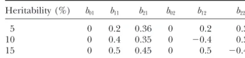
Heritability (%) b01 b11 b21 b02 b12 b22 The overall log-likelihood of the entire mapping

popu-5 0 0.2 0.36 0 0.2 0.36

lation is

10 0 0.4 0.35 0 ⫺0.4 0.35

15 0 0.5 0.45 0 0.5 ⫺0.45

L(␪)⫽

兺

n

j⫽1

ln[Pr(wj1,yj1|␪)]. (30)

Again, we adopt the EM algorithm to find the MLE

RESULTS of parameters. The maximization step is accomplished

through Equations 13 and 14. The expectation step _{Simulation studies:}To further evaluate the properties requires calculation of the posterior probabilities of of the proposed method, we conducted two simulation QTL genotypes and then uses these probabilities to find experiments. For the sake of simplicity, we designed one various expectations. The posterior probability of a QTL experiment to evaluate the performance of joint

map-genotype is ping for two binary traits and another experiment for

the mixture of one binary and one quantitative trait. In pjq* ⫽Pr(xj⫽ hq|IM,wj1,yj1)

each experiment, one chromosome with 11 evenly dis-tributed markers was simulated for an F2 population. ⫽ pjqPr(wj1,yj1|hqB,R)

兺

3

h⫽1pjhPr(wj1,yj1|hhB,R)

, ₍₃₁₎

We simulated a single QTL located at 35 cM of the chromosome and the QTL effects of both traits under from which we get the expectations

three different levels of heritability (proportion of vari-ance in liability explained by the QTL). The effects of

兺

n

j⫽1

E(xT

jxj)⫽

兺

n

j⫽1

⎡ ⎢

⎣

兺

3

q⫽1

pjq*hTqhq

⎤ ⎥

⎦ the QTL used in the simulation experiments are givenin Table 1. The correlation coefficient between the re-siduals of the liabilities for the two traits was chosen at 0.25. Under these settings, both traits had the same

兺

n

j⫽1

E(xT

jyj)⫽

兺

n

j⫽1

⎡ ⎢

⎣

兺

3

q⫽1

pjq*hTqE(yj|wj1,hq,␪)

⎤ ⎥ ⎦

, (32)

heritability. The three levels of the QTL effects led to three different levels of the heritability: 5, 10, and 15%. where

The genetic correlation between the two traits was ex-E(yj|wj1,hq,␪)⫽

关

E(yj1|wj1,hq,␪,yj1) yj1

兴

(33) pected to be 1.0, ⫺0.446, and 0.423, respectively, for the different chosen levels of the heritability. The sam-is a 1 ⫻ m vector, which has been partitioned into a

ple size of the simulated F2 population was n ⫽ 200. scalarE(yj1|wj1,hq,␪,yj1) and a vectoryj1. The

expecta-Each simulation experiment was replicated 100 times. tion is taken only for the liability of the binary trait. The

The first simulation experiment was to evaluate the remaining traits already take the observed values and

efficiency of the joint binary trait mapping. We first thus no expectations are taken. The expectation for the

simulated the liabilities of the two traits and then artifi-liability, E(yj1|wj1,hq,␪,yj1), is obtained from the

trun-cially truncated the continuous liabilities into two binary cated normal distribution with mean given by Equation

phenotypes using a threshold of zero. In the second B5 of appendix b and variance given by Equation B6

simulation experiment, we truncated only the liability ofappendix b. The residual error covariance matrix is

of the first trait to generate a binary phenotype but left given by Equation 18. However, the conditional

expecta-the second trait intact so that we had one binary trait tion is replaced by

and one continuous trait.

␮jq⫽E(yj|wj1,hq,␪) (34) Each data sample was analyzed using both the joint-mapping and single-trait-joint-mapping statistics. For the sin-and the conditional variance by

gle-trait analysis, we usedLanderandBotstein’s (1989) method for the continuous trait and the method ofXu

et al. (2003) for the binary trait. Since we considered only two traits in the joint mapping, explicit formulas were used in each of the EM iteration steps (see appen-dix afor the explicit formulas). The critical values for the chromosomewise type I error rate of 5% were deter-mined by the approximate method ofPiepho(2001). (35)

In real data analysis, one should use the permutation where Var(yj1|wj1,hq,␪,yj1) is the variance of a

trun-test (ChurchillandDoerge1994) to obtain the most cated normal distribution. BothE(yj1|wj1,hq,␪,yj1) and

appropriate critical values for significance tests. For the Var(yj1|wj1,hq,␪,yj1) can be found from the truncated

joint analysis, the empirical power was determined by normal distribution (Cohen1991) and no Gibbs

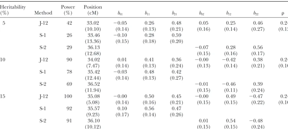
TABLE 2

Comparison of joint mapping with single trait mapping from the first simulation experiment (both traits are binary)

Heritability Power Position

(%) Method (%) (cM) b01 b11 b21 b02 b12 b22 ␳

5 J-12 42 33.02 ⫺0.05 0.26 0.48 0.05 0.25 0.46 0.24

(10.10) (0.14) (0.13) (0.21) (0.16) (0.14) (0.27) (0.13)

S-1 26 33.46 ⫺0.10 0.28 0.59

(13.36) (0.15) (0.18) (0.20)

S-2 29 36.13 ⫺0.07 0.28 0.56

(12.68) (0.15) (0.16) (0.17)

10 J-12 90 34.02 0.01 0.41 0.36 ⫺0.00 ⫺0.42 0.38 0.24

(7.47) (0.14) (0.13) (0.24) (0.13) (0.14) (0.21) (0.10)

S-1 78 35.42 ⫺0.03 0.48 0.42

(12.44) (0.14) (0.13) (0.27)

S-2 69 36.52 ⫺0.01 ⫺0.46 0.39

(11.94) (0.15) (0.11) (0.24)

15 J-12 100 35.08 ⫺0.00 0.50 0.45 ⫺0.00 0.49 ⫺0.47 0.24

(5.08) (0.14) (0.16) (0.21) (0.15) (0.15) (0.22) (0.10)

S-1 92 35.57 0.10 0.56 0.47

(9.23) (0.17) (0.14) (0.26)

S-2 91 36.10 0.01 0.54 ⫺0.48

(10.12) (0.15) (0.15) (0.24)

Entries for the QTL effect and location estimates are the average of 100 replicated simulations with the standard deviations among the 100 replicates given in parentheses. J-12, joint mapping; S-1, separate mapping for trait 1; S-2, separate mapping for trait 2.

whose highest test statistic values along the chromosome wherep1andp2are the powers for traits 1 and 2, respec-tively, andp12is the proportion of the replicated simula-were greater thanPiepho’s (2001) critical value. The

peak where the highest test statistic occurred was usually tions in which both traits are significant. For example, among the 100 replicates, if a significant QTL effect is close to the true QTL position. However, a significant

QTL was declared even if the peak was not exactly at detected in 50 samples for the first trait and a significant QTL effect is detected in 80 samples for the second the true position. For the separate analyses of individual

traits, the statistical power was determined for the analy- trait, thenp1⫽0.5 andp2⫽0.8. If QTL effects for both traits are detected in 40 samples, then p12⫽ 0.4. The sis of each trait as in the joint analysis. The critical value

was recalculated for each trait in each replicate. combined power for the separate analyses will be 0.5⫹ 0.8⫺0.4⫽0.9. Using this approach to calculating the Tables 2 and 3 show the observed powers of QTL

de-tection, the mean, and standard deviations (SD) of the power, the combined power of the separate trait analyses was almost identical to that of the joint analysis (data estimated QTL locations and effects obtained from 100

replicated simulations. We compared the power of the not shown). Therefore, power increase in joint mapping as opposed to separate mapping depends on how one joint analysis with that of a single-trait analysis for each

trait separately. Joint analysis has a substantially higher defines the power in the separate analyses. From the traditional definition of statistical power for single-trait power than either single-trait analysis. We understand

that this may not be a fair comparison because joint analysis (JiangandZeng1997), joint analysis has higher power than single-trait analysis,i.e., joint power greater analysis uses two traits while the single-trait analysis uses

only one trait. However, this has been the standard way than p1 and joint power greater thanp2. But the joint analysis has an equivalent power to the combined power for comparison of joint mapping with separate mapping

(JiangandZeng1997). One may want to redefine the for separate analyses if the combined power is defined asp1⫹ p2⫺p12,i.e., joint power⬇p1⫹ p2⫺ p12. power for the separate analyses as the ability to detect

at least one QTL effect (either additive or dominance) The QTL effects and their standard deviations esti-mated from the joint mapping are comparable to those in at least one trait. Under this definition of the power,

results of the two separate analyses may be combined obtained from separate analyses. No obvious advantage of the joint mapping has been demonstrated from the so that the power is recalculated in the combined result.

The combined power analysis requires either redefining simulation studies with respect to the estimates of QTL effects. The real advantage of the joint mapping over the critical values by taking into account the multiple

tests, which is difficult because the two separate analyses separate analyses has been demonstrated by the in-creased precision of the QTL position estimates in all may be highly correlated, or simply using the sum of the

powers of separate analyses (with an appropriate adjust- situations examined (see Tables 2 and 3).

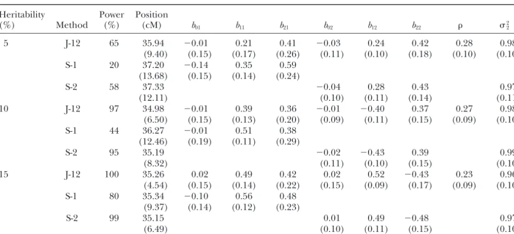
TABLE 3

Comparison of joint mapping with single trait mapping from the second simulation experiment (one binary trait and one quantitative trait)

Heritability Power Position

(%) Method (%) (cM) b01 b11 b21 b02 b12 b22 ␳ ␴22

5 J-12 65 35.94 ⫺0.01 0.21 0.41 ⫺0.03 0.24 0.42 0.28 0.98

(9.40) (0.15) (0.17) (0.26) (0.11) (0.10) (0.18) (0.10) (0.10)

S-1 20 37.20 ⫺0.14 0.35 0.59

(13.68) (0.15) (0.14) (0.24)

S-2 58 37.33 ⫺0.04 0.28 0.43 0.97

(12.11) (0.10) (0.11) (0.14) (0.11)

10 J-12 97 34.98 ⫺0.01 0.39 0.36 ⫺0.01 ⫺0.40 0.37 0.27 0.98

(6.50) (0.15) (0.13) (0.20) (0.09) (0.11) (0.15) (0.09) (0.10)

S-1 44 36.27 ⫺0.01 0.51 0.38

(12.46) (0.19) (0.11) (0.29)

S-2 95 35.19 ⫺0.02 ⫺0.43 0.39 0.99

(8.32) (0.11) (0.10) (0.15) (0.10)

15 J-12 100 35.26 0.02 0.49 0.42 0.02 0.52 ⫺0.43 0.23 0.96

(4.54) (0.15) (0.14) (0.22) (0.15) (0.09) (0.17) (0.09) (0.10)

S-1 80 35.34 ⫺0.10 0.56 0.48

(9.37) (0.14) (0.12) (0.23)

S-2 99 35.15 0.01 0.49 ⫺0.48 0.97

(6.49) (0.10) (0.11) (0.15) (0.10)

Entries for the QTL effect and location estimates are the average of 100 replicated simulations with the standard deviations among the 100 replicates given in parentheses. J-12, joint mapping; S-1, separate mapping for trait 1; S-2, separate mapping for trait 2.

true parametric values. The general trend follows our defined as w ⫽ 0 if the average score was within the range 0–3 andw⫽1 if the average score was 4–5. We expectation: high heritability tends to produce more

accurate estimates than low heritability. If we compare were provided only with the binary data, not the original scores. The breeders were more interested in the ge-the joint mapping of two binary traits with that of one

binary and one continuous trait, we will note the power netic study of the qualitative dichotomous trait than in the genetic study of the numerical scores. This explains difference between the two experiments. Experiment 2

shows higher powers than experiment 1. This observa- why we were approached by the breeders to analyze their data using the new methods.

tion also follows our expectation because binary data

are not as informative as continuously distributed data. Since the mapping population was a RIL population, a slight modification of our method for F2was required.

Mapping rice blast resistance loci:Developing blast

resistance cultivars is one of the major objectives in rice We replaced the probability transition matrix of F2 by that of F10in calculating the conditional probability of (Oryza sativa L.) breeding in both tropical and

temper-ate countries. The causal organism of the rice blast, QTL genotype (JiangandZeng1997). There was still a 4% residual heterozygosity in the RIL lines (due to Pyricularia grisea, is known for its high genetic variability,

allowing it to overcome the resistance of the host plant. F10instead of F∞), which is sufficiently high to allow the dominance effects to be estimated. We treated the plant A framework linkage map was developed using 284 F10

recombinant inbred lines (RILs) from a “Lemont” ⫻ responses to blast pathogen races IB54 and IG1 as two separate binary traits. Therefore, joint mapping for both “Teqing” rice cultivar cross. A subset of 245 RILs

innocu-lated with two rice blast races, IB54 and IG1, was used traits and separate mappings for individual traits were conducted for comparisons. The critical values of test to map loci responsible for the hypersensitive reaction.

Details of the experimental design, the measurements of statistics used to declare QTL were calculated using the method ofPiepho(2001).

phenotypes, and genotypes can be found in the original

article by Tabien et al. (2000). The phenotypes were Table 4 shows the results of joint mapping and sepa-rate analyses. The joint mapping may have a greater evaluated using a completely randomized design with

three replicates. In other words, each line was evaluated power than separate analyses, as demonstrated by more detected QTL and higher test statistic values. A total of three times for its reaction to each of the phathogen

infections. The original scores of the plant response five resistance loci were identified by the joint mapping (qtl1–qtl5), but only four of them were detected with were measured from grade 0 to grade 5. The average

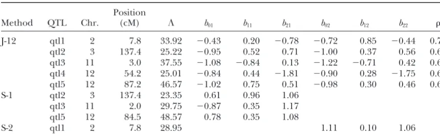
TABLE 4

QTL mapping result for rice blast resistance in the “Lemont”⫻“Teqing” crossing experiment

Position

Method QTL Chr. (cM) ⌳ b01 b11 b21 b02 b12 b22 ␳

J-12 qtl1 2 7.8 33.92 ⫺0.43 0.20 ⫺0.78 ⫺0.72 0.85 ⫺0.44 0.73 qtl2 3 137.4 25.22 ⫺0.95 0.52 0.71 ⫺1.00 0.37 0.56 0.65 qtl3 11 3.0 37.55 ⫺1.08 ⫺0.84 0.13 ⫺1.22 ⫺0.71 0.42 0.63 qtl4 12 54.2 25.01 ⫺0.84 0.44 ⫺1.81 ⫺0.90 0.28 ⫺1.75 0.69 qtl5 12 87.2 46.57 ⫺1.02 0.75 0.51 ⫺0.98 0.30 0.46 0.66

S-1 qtl2 3 137.4 23.35 0.61 0.96 1.06

qtl3 11 2.0 29.75 ⫺0.87 0.35 1.17

qtl5 12 84.5 48.57 0.78 0.35 1.08

S-2 qtl1 2 7.8 28.95 1.11 0.10 1.06

⌳is the likelihood-ratio test statistic and␳is the residual correlation. J-12, joint mapping for IB54 and IG1; S-1, separate mapping for IB54; S-2, separate mapping for IG1. The critical values of the test statistic (Piepho 2001) used to declare QTL were 20.57 for the J-12 analysis and 18.15 for each of the separate analyses (S-1 and S-2). Chr., chromosome.

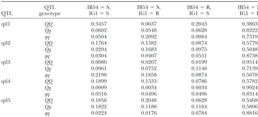
toPi-tq5,Pi-lm2, and Pi-tq6detected previously on the listed the probabilities of all the four possible phenotype combinations for all genotypes of each detected QTL basis of chi-square tests of individual marker-trait

associ-ations (Tabien et al. 2000). Two additional loci (qtl2 in Table 5. The penetrances of any particular genotypes for each QTL may be calculated from this table. For and qtl5) were detected on chromosomes 3 and 12, and

they were not reported in the previous study (Tabien example, if we define the penetrance of a genotype as the probability that a plant with this genotype is affected et al. 2000). For each of the two loci, the allele carried

by the Lemont parent was responsible for the resistance. by either of the two pathogens, the penetrance should be calculated using 1 ⫺ Pr(IB54 ⫽ R and IG1 ⫽ R). None of the genetic parameters,e.g., the QTL effects

and positions, were estimable in the previous chi-square On the other hand, if we define the penetrance as the probability that the plant is affected by both pathogens, tests conducted by the original authors (Tabien et al.

2000). The most striking result from the joint mapping then we should use Pr(IB54 ⫽ S and IG1 ⫽ S). The marginal penetrance for one pathogen, say pathogen was that all five resistance loci showed fairly consistent

effects against bothP. grisearaces, while different resis- IB54, should be defined as tance loci were detected separately by the single-trait

Pr(IB54⫽S)⫽Pr(IBS⫽ S and IG1⫽S) analyses.

It is worth mentioning that results of joint mapping ⫹ Pr(IBS⫽S and IG1⫽ R). and separate mapping do not seem to be consistent in

Taking the first genotype of the first QTL, for example, the real data analyses. This inconsistency, however, did

we may be able to find penetrances defined in all possi-not occur in the simulation studies. The reason for this

ble ways, as shown below, is that we have taken a one-dimensional genome-scan

approach, which uses a single-QTL model. In the simula- _{Pr(affected by either pathogen|QQ)⫽1⫺Pr(IB54⫽R and IG1⫽R)} tion studies, we indeed simulated a single QTL. There- _{⫽1⫺0.3863⫽0.6137,}

fore, the model adequately described the data. In the _{Pr(affected by both pathogens|QQ)⫽Pr(IB54⫽S and IG1⫽S)}

real data analysis, however, we used the single-QTL _⫽0.3457,

model to fit data controlled by apparently multiple QTL. _{Pr(affected by IB54|QQ)⫽Pr(IB54⫽S)}

The remaining QTL not fitted in the model may have _{⫽Pr(IB54⫽S and IG1⫽S)} caused all the inconsistencies observed between the _{⫹Pr(IB54⫽S and IG1⫽R)} joint and the separate analyses. In addition, the back- _{⫽0.3457⫹0.0637⫽0.4094,} ground QTL also have caused the observed high

resid-and ual correlation. These problems can be solved by fitting

a multiple-QTL model (see the discussion in a later _{Pr(affected by IG1|QQ)⫽Pr(IG1⫽S)}

section). _{⫽Pr(IB54⫽S and IG1⫽S)}

Table 5 shows the probabilities of the four possible _{⫹Pr(IB54⫽R and IG1⫽S)} phenotypic combinations under different genotypes of _{⫽0.3457⫹0.2043⫽0.55.} the identified QTL. For a single disease trait, penetrance

is defined as the probability that a specific QTL geno- Interested rice geneticists and breeders may want to find out all kinds of penetrances of interest from Ta-type shows the affected phenoTa-type. Penetrance has not

TABLE 5

The penetrances of QTL genotypes for rice blast resistance in the “Lemont”⫻“Teqing” crossing experiment

QTL IB54⫽S, IB54⫽S, IB54⫽R, IB54⫽R,

QTL genotype IG1⫽S IG1⫽R IG1⫽S IG1⫽R

qtl1 QQ 0.3457 0.0637 0.2043 0.3863

Qq 0.0602 0.0548 0.0628 0.8222

qq 0.0504 0.2092 0.0084 0.7319

qtl2 QQ 0.1764 0.1582 0.0874 0.5779

Qq 0.2294 0.1683 0.0975 0.5048

qq 0.0304 0.0407 0.0551 0.8738

qtl3 QQ 0.0080 0.0207 0.0199 0.9514

Qq 0.0961 0.0752 0.1148 0.7139

qq 0.2190 0.1858 0.0874 0.5078

qtl4 QQ 0.1899 0.1533 0.0786 0.5782

Qq 0.0009 0.0034 0.0034 0.9924

qq 0.0516 0.0496 0.0496 0.8314

qtl5 QQ 0.1856 0.2048 0.0628 0.5468

Qq 0.1822 0.1188 0.1184 0.5806

qq 0.0224 0.0176 0.0784 0.8816

R, resistance; S, susceptibility.Qrepresents the allele from parent “Lemont” andqrepresents the allele from parent “Teqing.”

an optimal marker-assisted seletion scheme to improve Atchley1996;YiandXu1999, 2000;Xuet al. 2003), using likelihood-based methods or Bayesian methods. blast resistance in rice.

However, the method of separate analyses of individual binary traits is, so far, the only approach currently avail-DISCUSSION _{able. For the first time, we developed the full probability} model for joint mapping of multiple binary traits. The Joint mapping offers several advantages over

single-method requires numerical multiple integrals, as we trait analyses. First, joint mapping may increase

statisti-know that high-dimensional numerical integration can-cal power of QTL detection compared to single-trait

not be implemented easily in practice. Therefore, we analyses. Second, joint analysis can improve the

preci-presented the method using two traits as examples. In sion of parameter estimation. Third, joint mapping

pro-real data analysis, one may pay more attention to the vides an opportunity to answer more questions related

information extracted from the data and thus may wish to the genetic architecture of complex traits. These have

to perform joint mapping for more than two traits using been discussed by many authors (JiangandZeng1995;

the general algorithm developed here. Two factors may Korolet al. 1995; Manginet al. 1998;Henshalland

limit the number of traits included in the analysis. One Goddard 1999; KnottandHaley 2000) in multiple

is the computing time and the other is the difficulty in quantitative traits QTL mapping. Similar advantages

interpreting the results. For the rice blast data analysis also have been demonstrated here in the joint mapping

with two binary traits, QTL search for the entire rice for multiple binary traits. In this study, we paid more

genome tookⵑ10 min, which is quite reasonable. For attention to the development of the EM algorithm

more than two traits, computing time is a big factor of rather than to various hypotheses tests, because the

lat-concern. We highly recommended using a different but ter have been fully addressed byJiangandZeng(1995).

fast numerical integration algorithm specially designed In addition, the method was derived in the context

for high-dimensional integration,e.g., Monte Carlo inte-of interval mapping. Extension to composite interval

gration. The Bayesian method implemented via Markov mapping should be preferred in practice, but this is

chain Monte Carlo (MCMC) is an ideal tool to accom-simply a matter of implementation. Furthermore, the

pro-plish this. In addition, the Bayesian method can handle posed method for F2populations can be easily extended

the multiple-QTL model with ease. To deal with the prob-to other types of populations,e.g., backcrosses or

four-lem of interpretation, one must have some intuitive way crosses, as demonstrated by the extension from F2

knowledge about the trait relationships and hypotheses to RILs described in this study. The method differs from

underlying the traits. In the disease-resistance case, one one mating design to another only by the possible

differ-would be interested not only in the number of loci ent number of genotypes and different transition matrix

involved, but also in the level of race specificity of indi-from one locus to another.

vidual resistance loci, since the hypersensitive response In fact, there has been much work on single binary

gene-for-gene system (Silue´et al. 1992). However, this gene- tween host plants and their pathogens in natural and agricultural systems (LeonardandCzochor1980). Joint for-gene system normally assumes that only two

conse-quences, resistance or susceptibility, would result from analyses of the correlated qualitative and quantitative phenotypes may substantially increase the power of de-interactions between alleles at a resistance locus of host

plants and alleles at its corresponding avirulence locus tecting disease resistance loci and allow exploration of in pathogens, which may not be always true, as is dis- new features of loci involved.

cussed in the following section; imperfect penetrance _{We are grateful to three anonymous reviewers for their suggestive} appears to be an important feature of resistance loci in- comments on early versions of the manuscript. This research was sup-ported by the National Institutes of Health grants R01-GM55321 and

volved in the gene-for-gene interactions between host

the United States Department of Agriculture National Research

Ini-plants and their pathogens.

tiative competitive grants program 00-35300-9245 to S.X.

We took the maximum-likelihood approach and im-plemented the method via the EM algorithm. This is different from the GEE method described earlier. We

favor the EM algorithm because it was developed on the LITERATURE CITED

basis of all existing theory and methods currently used _{Anderson, T. W., 1984 An Introduction to Multivariate Statistical} Analy-for mapping loci of regular quantitative traits. In single sis, Ed. 2. Wiley, New York.

Chan, J. S. K., and A. C.Kuk, 1997 Maximum likelihood estimation

binary trait mapping, one of the most frequently asked

for probit-linear mixed models with correlated random effects.

questions is “What is the advantage of using the proba- _{Biometrics88:86–97.}

bility model over the simple analysis that treats the bi- Churchill, G. A., and R. W. Doerge, 1994 Empirical threshold values for quantitative trait mapping. Genetics138:963–971.

nary traits as if they were continuous traits?” (Visscher

Cohen, A. C., 1991 Truncated and Censored Samples. Marcel Dekker, et al. 1996). The same question also may be asked here _{New York.}

for joint mapping of multiple binary traits. Although DeGroot, M. H., 1986 Probability and Statistics. Addison-Wesley, Reading, MA.

we did not try the joint analysis of binary traits by

ignor-Dempster, A. P., N. M. Lairdand D. B.Rubin, 1977 Maximum

ing the binary nature of the traits, we predict that treat- _{likelihood from incomplete data via the EM-algorithm. J. R. Stat.} ing binary traits as if they were continuous traits may Soc.39:1–38.

Devroye, T., 1986 Non-Uniform Random Variable Generation.

Springer-result in similar power in most situations. In some

spe-Verlag, New York.

cial cases, the probabilistic model may provide higher _{Diggle,A. P., K.-Y.Liangand S. L.Zeger, 1996 Permutation tests} power than the simplified analysis, and we have not _{for multiple loci affecting a quantitative character. Genetics142:}

285–294.

figured out the parameter range in which this will

hap-Giri, N. C., 1996 Multivariate Statistical Analysis. Marcel Dekker, New

pen. The probabilistic model approach enables

estima-York.

tion of penetrance of a particular QTL genotype, which _{Gueorguieva, R. V., and A. Agresti, 2001 A correlated probit}

model for joint modeling of clustered binary and continuous

is an important property of genes involved in human

responses. J. Am. Stat. Assoc.96:1102–1112.

diseases (TerwilligerandWeiss1998) and plant

dis-Hackett, C. A., and J. I.Weller, 1995 Genetic mapping of

quantita-ease resistance, as we demonstrated here.McIntyreet al. _{tive trait loci for traits with ordinal distributions. Biometrics51:} (2001) developed a different probabilistic model for 1252–1263.

Hackett, C. A., R. C.Meyerand W. T. B.Thomas, 2001

Multi-QTL mapping of binary traits. The method also allows

trait QTL mapping in barley using multivariate regression. Genet.

calculation of penetrance. Extension of their model to _{Res.77:95–106.}

multiple binary trait analysis is another alternative ap- Henshall, J. M., and M. E.Goddard, 1999 Multiple trait mapping of quantitative trait loci after selective genotyping using logistic

proach. We did not choose this extension because the

regression. Genetics151:885–894.

threshold model via the EM algorithm has a natural _{Huang, J., and Y. M.Jiang, 2003 Genetic linkage analysis of a} dichot-connection to existing methods of QTL mapping. omous trait incorporating a tightly linked quantitative trait in

affected sib pairs. Am. J. Hum. Genet.72:946–960.

Finally, with the successful development of joint

map-Jiang, C., and Z-B.Zeng, 1995 Multiple trait analysis of genetic

ping of both multiple quantitative and qualitative traits, _{mapping for quantitative trait loci. Genetics140:1111–1127.} an important but largely unexploited area in genetic Jiang, C., and Z-B.Zeng, 1997 Mapping quantitative trait loci with

dominant and missing markers in various crosses from two inbred

mapping begins to emerge,i.e., the joint analysis of mixed

lines. Genetica101:47–58.

types of traits. Although some authors (Williamset al. _{Knott, S. A., and C. S.Haley, 2000 Multitrait least squares for} 1999;HuangandJiang2003) already exploited this idea quantitative trait loci detection. Genetics156:899–911.

Korol, A. B., Y. T.Roninand V. M.Kirzhner, 1995 Interval

map-in the context of human genetic mappmap-ing under the

ping of quantitative trait loci employing correlated trait

com-IBD-based random model framework, it has never been

plexes. Genetics140:1137–1147.

explored in QTL mapping of experimental populations. Korol, A. B., Y. T.Ronin, A. M.Itskovich, J.Pengand E.Nevo, 2001 Enhanced efficiency of quantitative trait loci mapping

The method may be particularly useful in situations where

analysis based on multivariate complexs of quantitative traits.

mapping qualitative disease resistance of the

gene-for-Genetics157:1789–1803.

gene system is the primary objective while traits associ- _{Lander, E. S., and S. D.Botstein, 1989 Mapping Mendelian factors}

underlying quantitative traits using RFLP linkage maps. Genetics

ated with quantitative resistance to the same or different

121:185–199.

pathogens are measured as by-products in the

experi-Lange, C., and J. C.Whittaker, 2001 Mapping quantitative trait loci

ment. This coexistence of qualitative and quantitative _{using generalized estimating equations. Genetics159:1325–1337.}

Leonard, K. J., and R. J.Czochor, 1980 Theory of genetic

be-tions among populabe-tions of plants and their pathogens. Ann. Tallis, G. M., 1963 The moment generating function of the trun-cated multi-normal distribution. J. R. Stat. Soc. Ser. B23: 223–229. Rev. Phytopathol.18:237–258.

Liang, K. Y., and S. L.Zeger, 1986 Longitudinal data analysis using Terwilliger, J. D., and K. M.Weiss, 1998 Linkage disequilibrium mapping of complex disease: Fantasy or reality? Curr. Opin. Bio-generalized linear models. Biometrika73:13–22.

Luo, Z. W., and M. J.Kearsey, 1992 Interval mapping of quantitative technol.9:578–594.

Visscher, P. M., C. S.Haleyand S. A.Knott, 1996 Mapping QTLs trait loci in an F2 population. Heredity69:236–242.

Mangin, B., P.Thoquetand N.Grimslev, 1998 Pleiotropic QTL for binary traits in backcross and F2 populations. Genet. Res.68:

55–63. analysis. Biometrics54:88–99.

McCulloch, C. E., 1994 Maximum likelihood variance components Williams, J. T., P.Van Eerdewegh, L.Almasyand J.Blangero, 1999 Joint multipoint linkage analysis of multivariate qualitative estimation for binary data. J. Am. Stat. Assoc.89:330–335.

McIntyre, L. M., C.Coffmanand R. W.Doerge, 2001 Detection and quantitative traits. I. Likelihood formulation and simulation results. Am. J. Hum. Genet.65:1134–1147.

and location of a single binary trait locus in experimental

popula-tions. Genet. Res.78:79–92. Xu, S., and W. R. Atchley, 1996 Mapping quantitative trait loci for complex binary diseases using line crosses. Genetics 143: Piepho, H. P., 2001 A quick method for computing approximate

thresholds for quantitative trait loci detection. Genetics 157: 1417–1424.

425–432. Xu, S., N. Yi, D. Burke, A. GaleckiandR. A. Miller, 2003 An SASInstitute, 1999 SAS/IML User’s Guide Version 8.SAS Institute, EM algorithm for mapping binary disease loci: application to Cary, NC. fibrosarcoma in a four-way cross mouse family. Genet. Res.82: Silue´, D., J. L.Notteghemand D.Tharreau, 1992 Evidence of a 127–138.

gene-for-gene relationships in theOryza sativa-Magnaporthe grisea Yi, N., and S.Xu, 1999 Mapping quantitative trait loci for complex pathosystem. Phytopathology82:577–580. binary traits in outbred populations. Heredity82:668–676. Tabien, R. E., Z. Li, A. H. Paterson, M. A. Marchetti, J. W. Stansel _Yi, N., and S.Xu, 2000 Bayesian mapping of quantitative trait loci

et al., 2000 Mapping of four major rice blast resistance genes _{for complex binary traits. Genetics155:1391–1403.} from ‘Lemont’ and ‘Teqing’, and evaluation of their

combina-torial effect for field resistance. Theor. Appl. Genet.101:1215–1225. Communicating editor: R.Doerge

APPENDIX A: MOMENTS OF TRUNCATED BIVARIATE NORMAL DISTRIBUTION

Let zT ⫽ _[z

1 z2] be a vector of two variables distributed as a standardized bivariate normal distribution with correlation␳. Let [a1,c1] and [a2,c2] be the double truncation points on variablesz1andz2, respectively, and define ␣1⫽Pr(z1⬎c1,z2⬎c2) as the area (integral) within the domain. Let us further define the first and second moments of the truncated standardized bivariate normal distribution atz1⬎ c1andz2⬎ c2as

E(z1)⫽

φ(c1)[1⫺ ⌽(d1)]⫹ ␳φ(c2)[1⫺ ⌽(d2)]

␣1

E(z2)⫽

φ(c2)[1⫺ ⌽(d2)]⫹ ␳φ(c1)[1⫺ ⌽(d1)]

␣1

E(z2

1)⫽ ␣ ⫹

c1φ(c1)[1⫺ ⌽(d1)]⫹ ␳2c2φ(c2)[1⫺ ⌽(d2)]⫹ ␳(1⫺ ␳2)φ2(c1,c2;␳) ␣1

E(z2

2)⫽ ␣ ⫹

c2φ(c2)[1⫺ ⌽(d2)]⫹ ␳2c1φ(c1)[1⫺ ⌽(d1)]⫹ ␳(1⫺ ␳2)φ2(c1,c2;␳) ␣1

E(z1z2)⫽ ␣␳ ⫹ ␳

c1φ(c1)⌽(d1)⫹ ␳c2φ(c2)⌽(d2)⫹(1⫺ ␳2)φ2(c1,c2;␳) ␣1

, _(A1)

where

d1⫽

c1⫺ ␳c2

√

1⫺ ␳2 (A2)

and

d2⫽

c2⫺ ␳c1

√

1⫺ ␳2

. _(A3)

Equations A1 can be found fromTallis(1963). Similarly, we can calculate the first and second moments of truncated standardized bivariate normal distribution at z1 ⬎ a1 and z2 ⬎ c2, z1 ⬎ a2 and z2 ⬎ c1, and z1 ⬎ a1 and z2 ⬎ a2, respectively. We further denote the above four truncated domains by 1, 2, 3, and 4, respectively. The following formula is used to calculate the moments under the double truncation with [a1,c1] and [a2,c2],

T⫽ ␣1T1⫹ ␣4T4⫺ ␣2T2⫺ ␣3T3

where Ti, i ⫽ 1, 2, 3, 4, represents the arbitrary first moment of (A1), ␣i represents the probability under the corresponding truncated domain, and

␣ ⫽

冮

c1 a1

冮

c2

a2

φ2(z1,z2;␳)dz1dz2⫽ ␣1⫹ ␣4 ⫺ ␣2⫺ ␣3. (A5)

APPENDIX B: CONDITIONAL EXPECTATION AND VARIANCE VIA GIBBS SAMPLER

The basic idea of the Gibbs sampler is to find the distribution of one element, sayyjk, conditional on the remaining components in vector yj and sample yjk from the conditional distribution. Under the assumption of multivariate normality for the liability vector,i.e.,yjⵑ Nm(xjB,R), the conditional density of a single component is univariate normal with mean and variance described as follows. First, let us make the following matrix partitioning, yj ⫽ [yjkyjk], where

yjk⫽[yj1. . . yj(k⫺1) yj(k⫹1). . .yjm] (B1)

is a special notation for a subset of vectoryj that excludes yjk; i.e., the subscript k indexes all elements exceptk. Using this special notation we can partition matrixBintoB⫽[bkBk], wherebTk ⫽ [b0kb1kb2k] is thekth column of matrixBand

Bk⫽[b1. . . bk⫺1 bk⫹1. . .bm] (B2)

is a submatrix ofBwith thekth column left out. Let us further partition matrixRinto

R ⫽

冤

Rkk Rkk

Rkk Rkk

冥

, (B3)

whereRkk⫽ 1,Rkk⫽[␳1k. . .␳(k⫺1)k ␳k(k⫹1). . .␳km], Rkk⫽ RTkk, and

(B4)

Note thatRkkis the submatrix ofRwith thekth row andkth column removed. The above matrix partitionings allow us to define the conditional mean ofyjkas

E(yjk|xj,␪,yjk)⫽xjbk⫹RkkR⫺kk1(yjk⫺xjBk)T (B5)

and the conditional variance as

Var(yjk|xj,␪,yjk)⫽Rkk⫺RkkR⫺kk1Rkk. (B6)

Having found the distribution of one component conditional on the remaining components, one can easily sample each element from its perspective univariate normal distribution. The binary phenotype for each trait has not played a role in the above sampling scheme. To incorporate this information, we need to sample each liability from a truncated normal distribution with the mean and variance given above. For example, ifwjk⫽0,yjkshould be sampled only ifyjkⱕ0. Ifwjk⫽1, however,yjkshould be sampled only ifyjk⬎0. In fact, we adopted the algorithm ofDevroye (1986) to simulate a variable from a truncated normal distribution. This special algorithm has a 100% rate of acceptance. The Monte Carlo sampling process is repeated many times with the simulatedyjforming a large sample,