DOI: 10.1534/genetics.109.100362
Expression Quantitative Trait Loci Mapping With Multivariate Sparse
Partial Least Squares Regression
Hyonho Chun* and Su
¨ndu
¨z Keles
x
*
,†,1*Department of Statistics and†Department of Biostatistics and Medical Informatics, University of Wisconsin,
Madison, Wisconsin 53705
Manuscript received January 2, 2009 Accepted for publication February 23, 2009
ABSTRACT
Expression quantitative trait loci (eQTL) mapping concerns finding genomic variation to elucidate variation of expression traits. This problem poses significant challenges due to high dimensionality of both the gene expression and the genomic marker data. We propose a multivariate response regression approach with simultaneous variable selection and dimension reduction for the eQTL mapping problem. Transcripts with similar expression are clustered into groups, and their expression profiles are viewed as a multivariate response. Then, we employ our recently developed sparse partial least-squares regression methodology to select markers associated with each cluster of genes. We demonstrate with extensive simulations that our eQTL mapping with multivariate response sparse partial least-squares regression (M-SPLS eQTL) method overcomes the issue of multiple transcript- or marker-specific analyses, thereby avoiding potential elevation of type I error. Additionally, joint analysis of multiple transcripts by multivariate response regression increases power for detecting weak linkages. We illustrate that M-SPLS eQTL compares competitively with other approaches and has a number of significant advantages, including the ability to handle highly correlated genotype data and computational efficiency. We provide an application of this methodology to a mouse data set concerning obesity and diabetes.
E
XPRESSION quantitative trait loci (eQTL)map-ping is a genetic mapmap-ping of genomewide gene expression. It combines traditional quantitative trait mapping and microarray technology. eQTL mapping provides an opportunity to investigate a large and unbiased set of traits that are immediately connected to DNA sequence variation; thereby it enables the study of gene networks. eQTL mapping studies have been
ap-plied in several model organisms and humans (Brem
et al. 2002; Schadt et al. 2003; Morley et al. 2004;
Chesleret al.2005; Strangeret al.2005; Wanget al.
2006). These studies have demonstrated several advan-tages of this line of research, from identifying candidate
genes (Schadt et al. 2003) to elucidating regulatory
networks (Bremet al.2002; Schadtet al.2003; Yvert
et al.2003).
Typical eQTL studies involve anN 3Gmatrix of gene
expression, where rows are different individuals (e.g.,
mice, in the order of tens) and columns are transcripts
(in the order of thousands), and anN3pmatrix (Xp)
with genomic marker (in the order of hundreds or more) information. eQTL analysis differs from tradi-tional quantitative trait loci (QTL) analysis in the
number of traits considered. We refer to Kendziorski
and Wang(2006) for a comprehensive review of general
statistical issues concerning eQTL studies. Initial meth-ods for eQTL mapping can be grouped into two (Kendziorskiet al.2006): (1) transcript-specific
analy-sis in which mapping of a single expression trait is considered at a time and the entire analysis consists of thousands of transcript-specific analyses and (2) marker-specific analysis in which differentially expressed tran-scripts are identified at a single marker (by considering a marker genotype as a treatment) and the complete analysis requires scanning for all the markers. Both approaches are multiple applications of traditional methods (QTL mapping and identification of differen-tially expressed transcripts) and are prone to elevation of the false positive rate. Moreover, these approaches analyze data disjointly, either at the transcript or the marker level, leading to loss of power.
Mapping methods based on a notion of meta-transcript, which combine multiple similarly behaving transcripts by clustering or principal components
anal-ysis of genomewide gene expression data (Lan et al.
2003; Yvert et al. 2003), are viable approaches for
reducing the number of tests and improving the power of linkage detection. However, these methods do not produce transcript-specific information because identi-fied markers associate with a meta-transcript and not with individual transcripts.
Supporting information is available online athttp://www.genetics.org/ cgi/content/full/genetics.109.100362/DC1.
1Corresponding author:Department of Statistics, University of Wisconsin,
1300 University Ave., Madison, WI 53705. E-mail: [email protected]
Recent efforts for eQTL analysis focus on combined analysis of all the transcript and marker data by collapsing the aforementioned approaches 1 and 2.
The mixture over markers (MOM) model of Kendziorski
et al.(2006) is the first approach to facilitate informa-tion sharing across transcripts by an empirical Bayes method. It identifies transcripts that map to at least one marker (mapping transcripts) and then characterizes one or more markers per mapping transcript by utilizing transcript-specific highest posterior density
regions. Recently, Gelfond et al. (2007) improved on
the MOM model by utilizing genomic locations of the transcripts. To identify mapping transcripts and related
eQTL simultaneously, Jia and Xu (2007) proposed a
shrinkage analysis through a Bayesian hierarchical model called BAYES. This approach treats eQTL map-ping in a variable selection context, where expression values of transcripts are modeled by linear functions of markers and variable selection is promoted by a special prior distribution specification, namely, the spike and
slab distribution (Mitchelland Beauchamp1988), on
regression coefficients. When fitting transcript-level regression models, BAYES uses all the transcripts and markers simultaneously to achieve better power in detecting linkages. These transcript-level regression models share the same set of prior distributions. Al-though BAYES is flexible enough to map multiple markers per transcript, it is highly parametric, relies on prior specifications, and requires intense computations. Furthermore, properties of BAYES when markers are highly correlated are not studied. This is an important practical challenge because markers in close proximity are often highly correlated due to linkage disequilib-rium (LD). These high correlations may hamper the performance of variable selection schemes that do not explicitly accommodate such a grouping structure.
In this article, we propose a multivariate response regression framework, named eQTL mapping with multivariate response sparse partial least-squares regres-sion (M-SPLS eQTL). We utilize sparse partial
least-squares (SPLS) regression (Chun and Kelesx2007), a
novel statistical methodology for multivariate response regression with built-in dimension reduction and vari-able selection. Such a formulation is motivated by the apparent power advantages of multiple phenotype modeling observed in traditional multitrait QTL
map-ping ( Jiangand Zeng1995; Allisonet al.1998). It aims
to capitalize on correlations between multiple tran-scripts while simultaneously dealing with all the markers. Recent computational models of eQTL
map-ping in the yeast Saccharomyces cerevisiae suggest that
most eQTL have weak effects and that half of transcripts require more than five loci (markers) under additive
models (Bremand Kruglyak2005). This study further
elucidated the importance of joint analysis of the multiple transcripts and markers to boost weak linkage signals. In our approach, we cluster genes into groups on
the basis of their expression similarity. This helps us to view the expression values within a cluster as a multivar-iate response. Then, we form a cluster-level multivarmultivar-iate response regression and employ SPLS regression to identify markers affecting all or a subgroup of genes within the cluster. In the next two sections, we review underlying principles of the SPLS regression by focusing on aspects important to our application and describe our
method in detail. In thesimulation studiessection, we
study the operating characteristics of our approach and compare it to other approaches. We show that the proposed framework has excellent power and very small type-I error and significantly outperforms its univariate
counterpart. In thecase study:application to mouse
data from a study of obesity and diabetessection,
we illustrate our approach with a mouse data set of
obesity and diabetes research (Lanet al.2006) and then
discuss potential extensions.
eQTL MAPPING WITH MULTIVARIATE SPLS REGRESSION
SPLS regression: Partial least-squares (PLS) regres-sion has been an alternative to ordinary least squares (OLS) regression in ill-conditioned linear regression models that arise in several disciplines such as chemistry,
economics, psychology, and pharmaceutical science (De
Jong1993). At the core of PLS regression is a dimension
reduction technique that operates under the assump-tion of a basic latent decomposiassump-tion of a response matrix
ðY 2 RN3qÞ
and a predictor matrixðX 2 RN3pÞ
,
Y ¼TQT1F; and X ¼TPT1E;
where T 2 RN3K is a matrix that produces
K linear
combinations (scores), P 2 Rp3K and
Q 2 Rq3K are
matrices of coefficients (loadings), andE 2 RN3p and
F 2 RN3qare matrices of random errors.
To specify the latent component matrixTsuch that
T¼XW, PLS requires finding the columns ofW¼(w1,
w2,. . .,wK) from successive optimization problems. The
criterion for the kth estimated direction vector wˆk is
formulated as
ˆ
wk¼argmaxwwTXTYYTXw
s:t:wTw ¼1; wTSXXwˆj¼0; ð1Þ
forj¼1,. . .,k1, whereSXXis the sample covariance
matrix ofX. After estimating the latent components (T),
loadings (Q) are estimated via OLS for the model
Y¼TQT1
F.bPLSis estimated by ˆbPLS¼W ˆˆQT, whereWˆ
andQˆare estimates ofWandQ, sinceY¼XWQT1
F¼
XbPLS1F.
In Chunand Kelesx(2007), we investigated
regression problems with a large number of variables, it suffers from the curse of dimensionality in the
contem-porary large p, small N setting. To address this, we
developed a sparse PLS regression that aims to promote
sparsity by imposing an L1penalty onto the direction
vector of PLS. The SPLS objective function is given by
min a;w ka
TMa1ð1kÞðwaÞTMðwaÞ1l
1jwj11l2jwj22
s:t:aTa¼1; ð2Þ
whereM¼XT
YYT
X. This formulation promotes an exact
zero property by imposing an L1 penalty onto a
surrogate of the direction vector (w) instead of the
original direction vector (a), while keeping a and w
close to each other. This formulation is discussed in
Chun and Kelesx(2007), where we also characterized
the solution of the minimization problem. The firstL1
penalty encourages sparsity on w, and the second L2
penalty takes care of potential singularity in M when
solving for w. The parameter k is for reducing the
concavity of the problem and avoiding locally optimal
solutions. We show in Chunand Kelesx(2007) that a
k-value of,0.5 performs well in practice and considering
multiple k-values has the effect of initiating the
algo-rithm with different starting values. After obtaininga
andw, we rescale the solution ofwto have norm 1 and
use this scaled version as the estimated direction vector. The direction vector objective function in (2) is utilized in the course of the SPLS algorithm to select
active (relevant) variables. We defineAto be an index
set for active variables,Kas the number of components,
andXAas the matrix of covariates of which indexes are
contained in A. Then, the computational SPLS
algo-rithm can be summarized as follows:
1. Set ˆbPLS¼0,A ¼ ;,k¼1, andY1¼Y.
2. While (k#K),
2.1. Findwˆby solving the minimization problem in (2)
withM ¼XTY
1Y1TX.
2.2. UpdateAasfi:wˆi6¼0g [ fi:bˆ
PLS i 6¼0g.
2.3. Fit PLS with XA by using k numbers of latent
components.
2.4. Update ˆbPLSby using the new PLS estimates of the
direction vectors, and update Y1 and k through
Y1)YXbˆ PLS
andk)k11.
As seen in formulation (2), SPLS has tuning
param-eters l1, l2, and K. Since this formulation becomes
highly singular whenq¼1 orY’s are highly correlated,
i.e., favorable scenarios for SPLS regression, we setl2to
‘with an elastic net penalty (Zouand Hastie2005).
This leads to the form of a soft thresholded estimator
(Chunand Kelesx2007). As a result, step 2.1 of the SPLS
algorithm takes the form of simple soft thresholding
driven only by l1. In principle, each direction vector
requires its own soft thresholding parameter. However,
tuning K numbers of parameters is computationally
prohibitive. Thus, we utilize the following adaptive form of a soft thresholded estimator where we need only to tuneh, 0# h #1:
˜
w¼ ðjwˆj hmax
1#i#pjwˆijÞIðjwˆj$ h1max#i#pjwˆijÞsignðwˆÞ:
This form of soft thresholding retains components that are greater than some fraction of the maximum
com-ponent. As a result, SPLS has two tuning parameters,h
andK, and these are tuned by cross-validation (CV).
SPLS regression can select a higher number of relevant variables than the available sample size since the number of variables that contribute to each di-rection vector is not limited by the sample size. This property is shared by recent variable selection methods
such as elastic net (Zou and Hastie 2005) and
supervised principal components (Bair et al. 2006).
Additionally, as apparent from the formulation in (2), SPLS regression is able to handle multivariate
Y 2 RN3q, q $ 1, without additional computational
complexity. This property motivates the use of SPLS regression within the context of eQTL mapping where the goal is to utilize transcript and marker information simultaneously.
M-SPLS eQTL: Our approach consists of two steps.
Step 1. Clustering of the G3 N expression matrix: Current
eQTL studies typically have a total ofNexperimental
units from two or more distinct populations. There is a vast literature on clustering of gene expression data. Among simple methods are nonparametric clustering
methods such as k-means, partitioning around
me-doids (Kaufmanand Rousseeuw1990), and
hierar-chical clustering (Eisen et al. 1998) or parametric
clustering methods such as a mixture of Gaussian
distributions (Fraley and Raftery 2002). We view
the choice of the clustering method as a design-dependent decision and present an example within our case study. The thrust of the clustering step is to provide a transition from transcript-level regression models to module/cluster-level regression models.
Step 2. Cluster-specific multivariate response SPLS regression with bootstrap confidence intervals: After the clustering/
grouping step, at each cluster k, we define a Gk
-dimensional response vector Yið:kÞ to denote the
expressions of all theGkgenes, measured on theith
subject. We then consider a cluster-specific marker model
Yið:kÞ¼Xi:BðkÞ1Ei:;
whereEi.denotes the random error matrix andB(k)is a
p 3 Gk matrix representing the contribution of each
markerm2{1,. . .,p} to the expression variation of each
transcript g2{1,. . .,Gk} of cluster k. Such a model is
Two apparent gains are expected from this approach. First, we expect it to be more powerful than both the individual transcript- and marker-specific analyses be-cause transcripts with similar patterns are considered simultaneously and correlations among the transcripts are taken into account. Thus, it will be able to detect weak linkages. Second, it is expected to avoid type-I error inflation by eliminating multiple model fittings. We illustrate these points with simulations. SPLS re-gression tends to select a set of highly correlated markers rather than a single one among them when the covariates that are collectively associated with a phenotype have a grouping structure. This group selection property is easily realized in the SPLS algo-rithm. The minimization problem in (2), with an
updated M in step 2.1, can allow a set of variables to
be admitted to the active setAsimultaneously in step
2.2. This property is especially attractive in the following two cases. First, when a region of the genome, covered
by a set of markers (e.g., in the form of haplotypes), is
associated with a phenotype, SPLS regression can localize the region rather than select a single marker from the set. Selecting the set of highly correlated markers is more desirable when the data do not dis-criminate among these due to small sample size. Second, when quantitative traits are linked to several physically linked loci with small effects, suggested by
several QTL mapping studies (reviewed in Flintet al.
2005), SPLS regression can capture these linked loci. The final stage of cluster-specific SPLS regression is constructing bootstrap confidence intervals for tran-script selection. The outcome of multivariate SPLS regression is a set of selected markers that significantly associate with one or more transcripts in the cluster and their estimated regression coefficients. We provide an example of such an outcome for a data set from our simulation study (simulation C-1) in Figure 1. Figure 1A depicts true linkages simulated for a cluster of 100 genes over 145 markers. Figure 1B displays linkages estimated by the SPLS regression. As evident in this plot, M-SPLS is able to select the true set of markers, but several false linkages, albeit with very small sizes, are also revealed for the selected markers. This is not realistic because, generally, a given marker or a set of markers is likely to associate with a subset of the genes within a cluster since cluster analysis is also prone to errors. To circumvent this, we construct bootstrap confidence intervals for transcript selection. After the initial appli-cation of M-SPLS regression, subjects are randomly selected with replacement and multivariate response PLS regression is fitted using only the selected markers from the original fit. An empirical distribution of estimated regression coefficients is obtained for each marker/transcript combination after a large number of bootstrap iterations. Using these empirical distribu-tions, a 95% confidence interval is constructed for each marker/transcript combination. The final summary of
linkages contains marker/transcript combinations for which the confidence intervals exclude zero. Figure 1C summarizes the linkages after the bootstrap confidence intervals are taken into account. Here, only the relevant transcripts have nonzero coefficients at the selected markers. For illustration purposes, we provide bootstrap confidence intervals for marker 137 (D18Mit123) across all 100 transcripts in Figure 1D.
SIMULATION STUDIES
We performed simulation studies to investigate the operating characteristics of M-SPLS eQTL by compar-ing it to available methods under various eQTL archi-tectures (simulations A and B). We paid attention to having both simple single-marker and more complex multiple-marker eQTL architectures. In addition, we allowed a large number of transcripts to be affected by a single architecture following some of the recent eQTL
mapping findings (Wuet al.2008). We also examined
the advantages of multivariate response SPLS regression by comparing it to its univariate counterpart (simula-tion C). In these simula(simula-tions, we inten(simula-tionally skipped the clustering step and treated all the transcripts as a group. However, the performance of multivariate re-sponse SPLS regression might depend on the compo-sition of a given cluster. In simulation C, we investigated the robustness of M-SPLS regression to different in-accuracies in cluster assignments and evaluated its ability to identify regions of the genome with a large
number of mapping transcripts,i.e., hotspots (Schadt
et al.2003).
Simulation A—comparison of M-SPLS eQTL to BAYES and MOM in the absence of a strong LD struc-ture among markers:We first compared M-SPLS eQTL
to BAYES ( Jiaand Xu2007) and MOM (Kendziorski
et al.2006) by adopting the simulation experiments of
Jiaand Xu(2007). Ten markers (p¼10) are generated
on a 360-cM genome by using the Haldane map
function (Haldane1919) and four eQTL are located
at markers 1, 3, 6, and 10. A total ofG¼1000 transcripts
and N ¼ 50 samples are generated following the
Bayesian regression model that forms the backbone of
Jiaand Xu’s (2007) BAYES method. In the first scenario
(A-1), each subgroup of transcripts is affected by only a single marker. Transcripts 1–50 are under the influence of marker 10, transcripts 601–604 of marker 3, tran-scripts 605–610 of marker 1, and trantran-scripts 961–1000 of marker 6. The remaining transcripts do not map to any markers and their expression values are determined by the error terms. eQTL control sizes, which are essen-tially coefficients of the relevant markers in the BAYES
regression model, are generated from N(0, 32), and
error terms are generated fromN(0, 0.12). In the second
by markers 1, 3, and 10, and transcripts 971–990 by markers 1 and 6. Data for the remaining transcripts as well as eQTL effects and error terms are generated as in the first scenario.
We generated 100 replicates of each simulation scenario and applied SPLS regression. We then com-pared the operating characteristics with the results
reported in Jia and Xu (2007). We note that Jia and
Xu(2007) use only 20 replicates, which is presumably
due to the computational complexity of the BAYES method. However, the results are overall comparable
because our results for 20vs.100 simulation replicates
are very similar. We used 99% bootstrap confidence
intervals based on 1000 bootstrap samples for transcript
selection whereas Jia and Xu (2007) use some
un-specified false discovery rate (FDR), which is>1%, for
linkage thresholding.
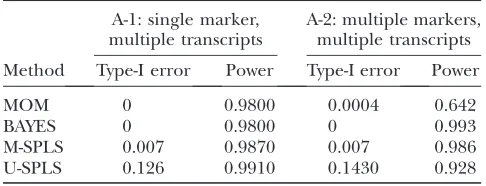
The simulation averages of power and type-I error are reported in Table 1. Here, U-SPLS refers to univariate SPLS regression where we fit an SPLS regression per transcript. U-SPLS is expected to produce many false positives due to multiple fitting of the regression model. As indicated in Table 1, indeed this approach has highly inflated type-I error. It is possible to argue that the performance of U-SPLS can be improved by implement-ing a bootstrap confidence interval step similar to that
Figure1.—(A) Set of true linkages. (B) Absolute values of the linkages estimated by M-SPLS regression. (C) Absolute values of
of M-SPLS. However, this increases computation time
considerably; i.e., if M-SPLS replicates 1000 bootstrap
samples, U-SPLS would replicate 1000 for eachGk
tran-script. We observe that M-SPLS has quite small type-I error and performs comparably to BAYES in terms of power despite the fact that the underlying data gener-ating model precisely follows the assumptions of BAYES. Additionally, we observe that M-SPLS has the ability to accommodate the case where multiple transcripts do not form a homogeneous group. This is a desired property since different groups of transcripts within a cluster could easily be associated with multiple-marker sets. We revisit this point in simulation C-2.
Simulation B—comparison of M-SPLS eQTL and BAYES with a strong LD structure among markers:The current literature on eQTL mapping utilizes a small number of markers that typically lack a strong LD structure when investigating operating characteristics
of methods by simulations (e.g., simulation A). In this
next set of simulations, we use all of the 145 markers
from 60 mice (p¼145 andN¼60) (Lanet al.2006) to
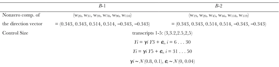
increase the number of markers and to reflect the ranges of LD structure that might exist among markers. We consider two types of eQTL architectures. In the first scenario (B-1), we select 6 markers (D2Mit17, D3Mit22, D4Mit190, D10Mit42, D12Mit217, and D13Mit66) ge-nomewide. This represents a case where the markers in the eQTL architecture do not necessarily have a grouping structure since these markers have a relatively low LD structure. In the second scenario (B-2), we select three chromosomes (2, 5, and 15) randomly, and 2
highly correlated adjacent markers per chromosome, depicting three eQTL covered by 6 markers (D2Mit274 at 69.6 cM, D2Mit17 at 73.9 cM, D5Mit259 at 43 cM, D5Mit9 at 46 cM, D15Mit193 at 58.4 cM, and D15Mit16 at 70.1 cM). In both B-1 and B-2, transcripts 1–5 are directly regulated by an architecture due to these 6 markers, components of which are described in
sup-porting information, Table S1. Transcripts 6–30 are
regulated by transcript 3, and transcripts 31–50 are regulated by transcript 5 to allow within-group correla-tion that is not due to markers. Remaining transcripts 51–60 are determined by a Gaussian error term. Average heritability across these 60 transcripts is 0.75. M-SPLS is tuned by 10-fold CV and we use 10,000 bootstrap samples for constructing confidence intervals. We use a cutoff of 0.2 for FDR control for BAYES.
As seen in Table 2, M-SPLS eQTL has significantly higher power than BAYES at the cost of a small increase in the type-I error. Power gain of M-SPLS eQTL is more noticeable in simulation B-2 with the strong LD struc-ture among the markers of the eQTL architecstruc-ture. This suggests that the grouping property of M-SPLS regres-sion could be beneficial in genetic mapping studies in the presence of linkages with strongly correlated mark-ers. Although this grouping property slightly increases the type-I error by including extra markers that have high correlations with the true set of relevant markers, SPLS starts to select a smaller set among the set of correlated markers as the sample size increases and the data start to discriminate these markers (simulation data not shown).
Simulation C—sensitivity of M-SPLS eQTL to the quality of cluster assignments: In simulations A-1 and A-2, we observed that M-SPLS regression overcomes the elevation of type-I error compared to U-SPLS by avoid-ing multiple model fits. However, the gain due to M-SPLS might depend on the quality of cluster assign-ments. Thus, we next compare performances of U-SPLS and M-SPLS regression by imposing different types of inaccuracies on cluster assignments. We consider two cases: (C-1) expression values of some of the cluster
transcripts are determined by noise, i.e., presence of
nonmapping transcripts, and (C-2) subgroups of tran-scripts within a cluster are controlled by different combinations of architectures. In addition, in simula-TABLE 1
Type-I error and power results based on the simulation setup of JIAand XU(2007)
A-1: single marker, multiple transcripts
A-2: multiple markers, multiple transcripts
Method Type-I error Power Type-I error Power
MOM 0 0.9800 0.0004 0.642
BAYES 0 0.9800 0 0.993
M-SPLS 0.007 0.9870 0.007 0.986 U-SPLS 0.126 0.9910 0.1430 0.928
TABLE 2
Type-I error and power results for simulation B
B-1: weak LDa B-2: strong LDa
Method Type-I error (SD) Power (SD) Type-I error (SD) Power (SD)
BAYES 0.009 (0.002) 0.832 (0.023) 0.004 (0.001) 0.612 (0.02) M-SPLS eQTL 0.014 (0.002) 0.915 (0.021) 0.008 (0.001) 0.942 (0.03)
tion C-3, we investigate the hotspot detection property of M-SPLS eQTL that is likely to be affected by the quality of cluster assignments.
Simulation C-1—noisy clusters with nonmapping tran-scripts:We assume that there is only one eQTL architec-ture involving several markers and affecting a percentage
of the genes in the cluster;i.e., the observed correlation
mechanism among the genes is a result of a single eQTL architecture. This corresponds to considering three
fac-tors in the data-generating scheme:r, number of relevant
markers in the eQTL architecture (3, 10);r, proportion
of cluster genes affected by the eQTL architecture (10,
30, 60, and 90%); and c, control size of the eQTL
architecture (weakvs.strong).
As in simulation B, we use the full set of markers from
60 mice. For each combination ofr,r, andc, we simulate
100 transcripts, treated as a group for M-SPLS regres-sion, as follows. We first generate a norm 1 eQTL
architecture direction vector with r nonzero
compo-nents. The sizes of the coefficients are controlled to a constant multiplied by this direction vector. We consider
the constantsc¼1 andc¼2 for weak and strong effects,
rproportion of transcripts are controlled by the eQTL
architecture, and random error terms are generated
fromN(0, 1). We use fivefold CV for marker selection
and 95% bootstrap confidence intervals based on 1000 bootstrap samples for transcript selection. The simulations are replicated 100 times. More details on data generation of these simulations are provided in Table S2.
Results are presented in Figure 2 in terms of power and type-I error. U-SPLS regression exhibits inflated type-I error as expected on the basis of the earlier
simulations following Jia and Xu’s (2007) design.
Additionally, the power of U-SPLS does not change as the proportion of transcripts associated with the eQTL mechanism increases. This is also expected since U-SPLS considers separate regression fits for each tran-script. On the other hand, M-SPLS regression has very small type-I error and, overall, has significantly higher power than U-SPLS. We note that in our data-generating scheme, the sizes of the coefficients are inherently
decreasing as the number of markers r in the eQTL
mechanism increases. This is because the sizes are proportional to the elements of the direction vector and the norm of the direction vector is by definition 1.
As a result, the r ¼ 10 markers and weak control
configuration have the highest noise level among the 16 configurations considered. Despite the decreasing overall signal at the transcript level, the power of
Figure2.—Results for
M-SPLS increases as the proportion of transcripts affected by the eQTL mechanism increases. This pro-vides evidence that M-SPLS successfully utilizes infor-mation across multiple transcripts; therefore, low signal linkages that might be missed by examining individual markers separately become detectable. Additionally, M-SPLS has more power than U-M-SPLS even when only 10% of the transcripts in the cluster are affected by the
same set of markers (at both control sizes whenr ¼
10).
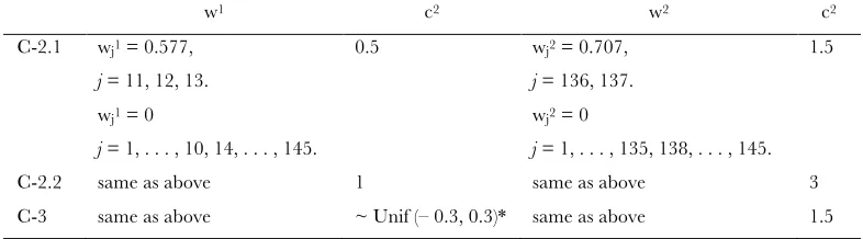
Simulation C-2—heterogeneous clusters with subgroups of transcripts controlled by different eQTL architectures: We next study the case where two hidden components, therefore two different eQTL architectures, are present.
These two components are (1)eQTL mechanism 1, linear
combinations of markers 11, 12, and 13; and (2)eQTL
mechanism 2, linear combinations of markers 136 and 137. Mechanism 1 is set to have a weaker control size than mechanism 2. We consider two cases for the multiple-eQTL architectures simulation:
C-2.1: Transcripts 1–50 are under the influence of mechanisms 1 and 2, and transcripts 51–90 are affected only by mechanism 1. Expression values of the rest of the transcripts are set by the error terms.
C-2.2: The same as C-2.1 but with a larger control size.
Details on the parameter settings are provided in Table S3.
Results of these multiple-eQTL architecture simula-tions are provided in Figure 3. M-SPLS has greater power than U-SPLS with a smaller type-I error. This observation is consistent with our earlier simulation experiments, suggesting that M-SPLS has the ability to accommodate cases where different groups of transcripts within a cluster are associated with multiple-marker sets.
Simulation C-3—clusters with weak eQTL effects:Hotspot regions are defined as loci of a genome that are mapped
by a large number of genes (Schadtet al.2003). They
lead to widespread changes in the expression of distant genes. Hotspots that exhibit strong control of their target transcripts are often easily identified with tran-script-specific approaches. However, if the hotspot locus exerts weak control over its targets, except maybe for
a few directly related transcripts (e.g., cis-regulation),
univariate approaches tend to miss these linkages and thus fail to identify the hotspot. In contrast, a multivar-iate approach might capture these weak linkages by utilizing correlations among transcripts.
Figure 3.—Results for
We assume that two subgroups of transcripts form a cluster and are controlled by different combinations of two architectures. Each of the architectures can be interpreted as hotspots as they control 50 and 80% of the transcripts. One of the architectures exerts weak control except for one transcript, but the other exhibits strong control of all linked transcripts. This setting is similar to that of simulation C-2.1 and more details are
provided inTable S3.
Figure 3 summarizes the results from this simulation. Linkages with the first eQTL mechanism cannot be detected by U-SPLS because the control size is very small, resulting in poor power for U-SPLS. In contrast, M-SPLS has at least twice the power of U-SPLS, although M-SPLS misses some of the linkages with this architec-ture. This result is also reflected in the hotspot selection performance of the methods. The first eQTL mecha-nism cannot be revealed as a hotspot from individual regression analyses by U-SPLS (Figure 3, bottom left). However, M-SPLS is able to identify markers involved in this mechanism as hotspots (Figure 3, bottom right).
CASE STUDY: APPLICATION TO MOUSE DATA FROM A STUDY OF OBESITY AND DIABETES
We present an application of our method to a mouse
data set published in Lan et al. (2006). This data set
contains expression measurements of 45,265 transcripts from liver tissues of 60 mice. Mice were collected from a
(B6 3 BTBR) F2-ob/ob cross where animals lacked a
functional leptin protein hormone, known to be im-portant for reproduction and regulation of body weight
and metabolism (Zhanget al.1994), and segregated for
obesity- and diabetes-related phenotypes. We utilized the preprocessed data that are publicly available at GEO (http://www.ncbi.nlm.nih.gov/projects/geo/query/acc. cgi?acc¼GSE3330). The marker map for these data consists of 145 microsatellite markers from 19 nonsex
mouse chromosomes. Following Jiaand Xu(2007), we
performed an initial screening of the transcripts on the basis of their variability across 60 mice and excluded
transcripts with sample variances ,0.12 from our
analysis. This left a total ofG¼1573 transcripts.
Next, we clustered these remaining transcripts. As discussed earlier, the clustering method in an application is highly design dependent. For a time-course experi-ment, methods that utilize dependencies among
differ-ent time points (Yuan and Kendziorski 2006) or
methods specifically parameterizing cluster profiles ( Jo¨ rnstenand Kelesx 2008) might be more desirable.
For the mouse data, we considered the following approach motivated by the successful use of the
topolog-ical overlap measure (TOM) (Ravasz et al. 2002) in
clustering analysis (Zhangand Horvath2005). First, we
constructed undirected, unweighted gene networks on the basis of the expression data, using the Gaussian
graphical model (GGM) approach of Scha¨ fer and
Strimmer(2005). The constructed network is then used
to compute TOM for each pair of transcripts. Dissimilar-ity measure 1-TOM between 2 transcripts represents a lack of closeness based on the number of shared neighbors in the expression network. Since 95 transcripts did not share any neighbors with other transcripts, they were analyzed by U-SPLS regression. Hierarchical clus-tering on the remaining transcripts using this dissimilar-ity measure resulted in 47 clusters based on the average
silhouette measure (Kaufman and Rousseeuw 1990).
The within-cluster Pearson correlations ranged from 0.027 to 0.948 with a mean of 0.226 across 47 clusters.
We present the results for one of the clusters in more detail. This cluster contains 3 lipid metabolism
tran-scripts, namely, Scd1, Elovl6, and Fasn, that were
in-vestigated by a different analysis of the same data set (Lanet al.2006; Jiaand Xu2007). There are a total of 83
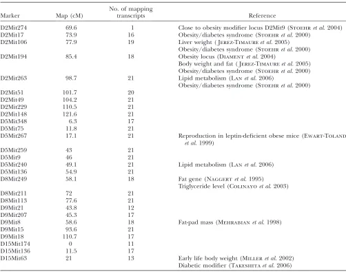
transcripts in this cluster with a median within-cluster correlation of 0.12. An application of our approach with M-SPLS yields 27 markers, presented in Table 3, that are associated with one or more transcripts. The total number of linkages identified for this cluster is 487 and there are 62 transcripts that do not map to any marker. An image plot of the estimated effects of this cluster across markers and transcripts is provided in Figure 4. The entire M-SPLS eQTL analysis, including both the tuning and the bootstrap steps, for this cluster of 83 transcripts took only 3 min on a 64-bit machine with 2.66-Ghz CPU.
We note that many of the selected markers are in close proximity to each other on the mouse genome. These physically close markers are highly correlated (pairwise correlations on chromosomes 2, 5, and 15 are displayed in Figure S1). The fact that these highly correlated markers are identified relates to the group selection property of the SPLS regression. Since SPLS can choose more than one variable at each step of the selection process, it is able to capture all the relevant correlated variables rather than arbitrarily selecting one. One can argue that, perhaps, the selected markers cover too large of a region on each chromosome. The problem of identifying such large regions is driven by the nature of the data. Since the markers are highly correlated, it is hard to select finer areas of the genome with data from
60 mice. Flintet al.(2005) argue that 300 F2animals are
needed to map a QTL with an effect size of 5% onto a 40-cM interval with 50% power, using markers that are spaced every 20 cM across the genome. We anticipate that more mice are needed to localize finer areas of the genome in eQTL studies. In each correlated marker group in Table 3, there is at least one marker that is previously declared as an obesity- and diabetes-related locus. This result is encouraging since it provides a list of transcripts mapping to markers known to be related to obesity and diabetes.
Expression profiles of lipid metabolism transcripts
plots are inFigure S2; minimum pairwise correlation is 0.756). Therefore, it is reasonable to expect similar linkages for these transcripts. Indeed, M-SPLS reveals that these transcripts map to similar markers, whereas BAYES yields different linkages. This could be due to high correlation among markers. Unlike the markers generated by the Haldane map function (simulations A-1 and A-2), markers from the mouse study exhibit very high correlations. This multicollinearity problem is not explicitly addressed in BAYES, and priors for regression coefficients are assumed to be independent. In fact,
similar mixture priors were used by Shaet al.(2006) in
the context of a different model and a decrease in the variable selection performance was observed for the correlated variable case. It is plausible that BAYES also suffers from a similar problem and tends to select only one variable among a set of correlated variables.
Lanet al.(2006) highlighted that transcripts that were
highly correlated withScd1mapped to the same genomic
locations asScd1, and found major QTL peaks for most of
the 20 lipid metabolism traits at markers D2Mit263 and D5Mit240. These two markers are successfully identified by our approach. Among the five hotspots reported by MOM, one of them is also identified by M-SPLS eQTL with the group of transcripts we considered. This is marker D8Mit249, which is close to the ‘‘fat’’ gene known to affect
obesity and diabetes (Naggertet al.1995). M-SPLS eQTL
identified D5Mit348, which is adjacent to D5Mit1, instead of D5Mit1, which affects triglyceride levels. Marker D15Mit63, emphasized in the findings of BAYES, is also identified by M-SPLS eQTL. Markers on chromosome 2 have been the most popular candidates for obesity and
diabetes (Stoehret al.2000; Diamentet al.2004; Jerez
-Timaureet al.2005), but hotspots from MOM and BAYES
do not have a noticeable indication of this. In particular, BAYES does not find any hotspots on chromosome 2. In contrast, M-SPLS eQTL yields strong effects for markers on chromosome 2. Furthermore, although marker TABLE 3
Markers identified for a cluster of size 83 including three lipid metabolism transcripts: Scd1, Elovl6, and Fasn
Marker Map (cM)
No. of mapping
transcripts Reference
D2Mit274 69.6 1 Close to obesity modifier locus D2Mit9 (Stoehret al.2004)
D2Mit17 73.9 16 Obesity/diabetes syndrome (Stoehret al.2000)
D2Mit106 77.9 19 Liver weight ( Jerez-Timaureet al.2005)
Obesity/diabetes syndrome (Stoehret al.2000)
D2Mit194 85.4 18 Obesity locus (Diamentet al.2004)
Body weight and fat ( Jerez-Timaureet al.2005)
Obesity/diabetes syndrome (Stoehret al.2000)
D2Mit263 98.7 21 Lipid metabolism (Lanet al.2006)
Obesity/diabetes syndrome (Stoehret al.2000)
D2Mit51 101.7 20
D2Mit49 104.2 21
D2Mit229 110.5 21
D2Mit148 121.6 21
D5Mit348 6.3 17
D5Mit75 11.8 21
D5Mit267 17.1 21 Reproduction in leptin-deficient obese mice (Ewart-Toland
et al.1999)
D5Mit259 43 21
D5Mit9 46 21
D5Mit240 49.1 21 Lipid metabolism (Lanet al.2006)
D5Mit136 54.9 21
D8Mit249 58.1 18 Fat gene (Naggertet al.1995)
Triglyceride level (Colinayoet al.2003)
D8Mit211 72 21
D8Mit113 77.6 21
D9Mit21 43.8 12
D9Mit207 45.3 17
D9Mit8 58.6 18 Fat-pad mass (Mehrabianet al.1998)
D9Mit15 93.6 21
D9Mit18 110.7 17
D15Mit174 0 11
D15Mit136 11.5 17
D15Mit63 21 13 Early life body weight (Milleret al.2002)
D5Mit267, which is identified by M-SPLS eQTL but missed by MOM and BAYES, does not seem to be directly related to obesity and diabetes, it is associated with reproduction, which is another known function of leptin
protein hormone (Ewart-Tolandet al.1999).
DISCUSSION
The advent of microarray technology is providing an unprecedented opportunity for investigating complex genetics underlying inheritance of transcript levels in segregating populations. One of the statistical chal-lenges is the eQTL mapping problem that concerns identification of linkages between thousands of tran-scripts and markers. We formulated the eQTL mapping problem as a variable selection problem in a multivar-iate response regression. We then utilized sparse partial
least squares (Chunand Kelesx2007) as a simultaneous
variable selection and dimension reduction approach to identify linkages. This framework, implemented as an
R package named SPLS (File S1), offers offers a
com-putationally fast alternative for analyzing multiple tran-script and marker data simultaneously to gain power and avoid multiplicities for good error control.
We demonstrated the advantages of our method with simulation experiments. These experiments included eQTL architectures with strong effects on a small fraction as well as weak effects on a large fraction of transcripts. These studies showed that as the number of mapping transcripts increases, the power of M-SPLS increases whereas its univariate analog with transcript-level regressions cannot capitalize on this phenomenon. We illustrated the utility of our approach with an
example from mouse obesity and diabetes research. This case study highlighted the ability of SPLS regres-sion to select groups of correlated markers. BAYES, an alternative variable selection approach to the eQTL problem, lacks this property and tends to select only one marker among the group of correlated markers. Our approach was able to consistently yield similar linkages for highly correlated transcripts. Furthermore, we were able to identify a marker that was missed by the previous analysis of the same data set but could potentially be important since it relates to another function of the
leptin protein hormone (Ewart-Tolandet al.1999).
In this article, we allowed the markers to appear as main terms in the regression model. Identifying inter-actions among markers is a challenging problem. With an appropriate prescreening of markers, SPLS regres-sion has the potential to handle a large number of
interactions. In Chunand Kelesx(2007), this property is
illustrated with as many as 5000 variables. Another important research question in eQTL mapping is allowing for linkages with locations between markers
using interval mapping (Chenand Kendziorski2007).
Our current formulation allows for mapping only at exact marker locations. However, a first pass with our approach and then a more focused traditional interval
mapping (Sen and Churchill 2001) based on the
selected markers might be a viable strategy.
We thank two anonymous referees for their constructive and valuable comments. This research has been supported in part by a Pharmaceutical Research and Manufactures of America Foundation Research Starter Grant in Informatics, by National Institutes of Health grant HG003747, and by National Science Foundation grant DMS 0804597 to S.K.
LITERATURE CITED
Allison, D. B., B. Thiel, P. S. Jean, R. C. Elston, M. C. Infanteet al.,
1998 Multiple phenotype modeling in gene-mapping studies of quantitative traits: power advantages. Am. J. Hum. Genet.63:
1190–1201.
Bair, E., T. Hastie, D. Pauland R. Tibshirani, 2006 Prediction by
supervised principal components. J. Am. Stat. Assoc.101:119– 137.
Brem, R., and L. Kruglyak, 2005 The landscape of genetic
com-plexity across 5700 gene expression traits in yeast. Proc. Natl. Acad. Sci. USA102:1572–1577.
Brem, R. B., G. Yvert, R. Clintonand L. Kruglyak, 2002 Genetic
dissection of transcriptional regulation in budding yeast. Science
296:752–755.
Chen, M., and C. Kendziorski, 2007 A statistical framework for
ex-pression quantitative trait loci (eQTL) mapping. Genetics177:
761–771.
Chesler, E. J., L. Lu, S. Shou, Y. Qu, J. Guet al., 2005 Complex trait
analysis of gene expression uncovers polygenic and pleiotropic networks that modulate nervous system function. Nat. Genet.
37:233–242.
Chun, H., and S. Kelesx, 2007 Sparse partial least squares regression
for simultaneous dimension reduction and variable selection.
http://www.stat.wisc.edu/keles/Papers/spls_jrssb.pdf. Colinayo, V. V., J. H. Qiao, X. P. Wang, K. L. Krass, E. Schadtet al.,
2003 Genetic loci for diet-induced atherosclerotic lesions and plasma lipids in mice. Mamm. Genome14:464–471.
deJong, S., 1993 SIMPLS: an alternative approach to partial least
squares regression. Chemometrics Intell. Lab. Syst.18:251–263.
Figure4.—M-SPLS solution for a cluster of 83 transcripts
Diament, A., P. Farahani, S. Chiu, J. Fislerand C. Warden, 2004 A
novel mouse chromosome 2 congenic strain with obesity pheno-types. Mamm. Genome15(6): 452–459.
Eisen, M. B., P. T. Spellman, P. O. Brown and D. Botstein,
1998 Cluster analysis and display of genome-wide expression patterns. Proc. Natl. Acad. Sci. USA95:14863–14868.
Ewart-Toland, A., K. Mounzih, J. Qiu and F. F. Chehab,
1999 Effect of the genetic background on the reproduction of leptin-deficient obese mice. Endocrinology140:732–738. Flint, J., W. Valdar, S. Shifmanand R. Mott, 2005 Strategies for
mapping and cloning quantitative trait genes in rodents. Nat. Rev. Genet.6:271–286.
Fraley, C., and A. E. Raftery, 2002 Model-based clustering,
discrimi-nant analysis, and density estimation. J. Am. Stat. Assoc.97:611–631. Gelfond, J. A. L., J. G. Ibrahimand F. Zou, 2007 Proximity model
for expression quantitative trait loci (eQTL) detection. Biomet-rics63:1108–1116.
Haldane, J. B. S., 1919 The combination of linkage values and the
calculation of distances between the loci of linked factors. J. Genet.8:299–309.
Jerez-Timaure, N. C., E. J. Eisenand D. Pomp, 2005 Fine mapping
of a QTL region with large effects on growth and fatness on mouse chromosome 2. Physiol. Genomics21:411–422. Jia, Z., and S. Xu, 2007 Mapping quantitative trait loci for
expres-sion abundance. Genetics176:611–623.
Jiang, C., and Z. Zeng, 1995 Multiple trait analysis of genetic
map-ping for quantitative trait loci. Genetics140:1111–1127. Jo¨ rnsten, R. J., and S. Kelesx, 2008 Mixture models with multiple
levels, with application to the analysis of multifactor gene expres-sion data. Biostatistics9:540–554.
Kaufman, L., and P. Rousseeuw, 1990 Finding Groups in Data: An Introduction to Cluster Analysis.John Wiley & Sons, New York. Kendziorski, C., and P. Wang, 2006 A review of statistical methods
for expression quantitative trait loci mapping. Mamm. Genome
17:509–517.
Kendziorski, C. M., M. Chen, M. Yuan, H. Lanand A. D. Attie,
2006 Statistical methods for expression quantitative loci (eQTL) mapping. Biometrics62:19–27.
Lan, H., J. P. Stoehr, S. T. Nadler, K. L. Schueler, B. S. Yandell et al., 2003 Dimension reduction for mapping mRNA abun-dance as quantitative traits. Genetics164:1607–1614.
Lan, H., M. Chen, J. B. Flowers, B. S. Yandell, D. S. Stapletonet al.,
2006 Combined expression trait correlations and expression quantitative trait locus mapping. PLoS Genet.2:e6.
Mehrabian, M., P. Z. Wen, J. Fisler, R. C. Davisand A. J. Lusis,
1998 Genetic loci controlling body fat, lipoprotein metabolism, and insulin levels in a multifactorial mouse model. J. Clin. Invest.
101:2485–2496.
Miller, R. A., J. M. Harper, A. Galeckiand D. T. Burke, 2002 Big
mice die young: early life body weight predicts longevity in genet-ically heterogeneous mice. Aging Cell1:22–29.
Mitchell, T. J., and J. J. Beauchamp, 1988 Bayesian variable
selec-tion in linear regression. J. Am. Stat. Assoc.83:1023–1036. Morley, M., C. M. Molony, T. M. Weber, K. G. Devlin, J. L. Ewens
et al., 2004 Genetic analysis of genome-wide variation in human gene expression. Nature430:743–747.
Naggert, J. K., L. D. Fricker, O. Varlamov, P. M. Nishina, Y.
Rouille et al., 1995 Hyperproinsulinaemia in obese fat/fat
mice associated with a carboxypeptidase E mutation which re-duces enzyme activity. Nat. Genet.10:135–142.
Ravasz, E., A. Somera, D. Mongru, Z. Oltvaiand A. Barabasi,
2002 Hierarchical organization of modularity in metabolic net-works. Science297:1551–1555.
Schadt, E. E., S. A. Monks, T. Drake, A. J. Lusis, N. Cheet al.,
2003 Genetics of gene expression surveyed in maize, mouse and man. Nature422:297–302.
Scha¨ fer, J., and K. Strimmer, 2005 Learning large-scale graphical
Gaussian models from genomic data, pp. 263–276 inAIP Confer-ence Proceedings 776. SciConfer-ence of Complex Networks: From Biology to the Internet and WWW (CNET 2004), edited by J. F. F. Mendes, S. N.
Dorogovtsev, F. V. A. A. Povolotskyand J. G. O. Ira. Aveiro,
Portugal. American Institute of Physics, Melville, NY.
Sen, S., and G. A. Churchill, 2001 A statistical framework for
quan-titative trait mapping. Genetics159:371–387.
Sha, N., M. G. Tadesseand M. Vannucci, 2006 Bayesian variable
selection for the analysis of microarray data with censored out-comes. Bioinformatics22:2262–2268.
Stoehr, J., S. Nadler, K. Schueler, M. Rabaglia, B. Yandellet al.,
2000 Genetic obesity unmasks nonlinear interactions between murine type 2 diabetes susceptibility loci. Diabetes49: 1946– 1954.
Stoehr, J. P., J. E. Byers, S. M. Clee, H. Lan, I. V. Boronenkovet al.,
2004 Identification of major quantitative loci controlling body weight variation in ob/ob mice. Diabetes53:245–249. Stranger, B. E., M. S. Forrest, A. G. Clark, M. J. Minichiello, S.
Deutschet al., 2005 Genome-wide associations of gene
expres-sion variation in humans. PLoS Genet.1:e78.
Takeshita, S., M. Moritani, K. Kunika, H. Inoueand M. Itakura,
2006 Diabetic modifier QTLs identified in F2 intercrosses be-tween akita and A/J mice. Mamm. Genome17:927–940. Wang, S., N. Yehya, E. E. Schadt, H. Wang, T. A. Drakeet al.,
2006 Genetic and genomic analysis of a fat mass trait with com-plex inheritance reveals marked sex specificity. PLoS Genet.2:
e15.
Wu, C., D. L. Delano, N. Mitro, S. V. Su, J. Janeset al., 2008 Gene
set enrichment in eQTL data identifies novel annotations and pathway regulators. PLoS Genet.4:e1000070.
Yuan, M., and C. Kendziorski, 2006 Hidden Markov models for
mi-croarray time course data in multiple biological conditions. J. Am. Stat. Assoc.101:1323–1332.
Yvert, G., R. B. Brem, J. Whittle, J. M. Akey, E. Foss et al.,
2003 Trans-acting regulatory variation inSaccharomyces cerevisiae
and the role of transcription factors. Nat. Genet.35:57–64. Zhang, B., and S. Horvath, 2005 A general framework for
weighted gene co-expression network analysis. Stat. Appl. Genet. Mol. Biol.4:Article 17.
Zhang, Y., R. Proenca, M. Maffei, M. Barone, L. Leopoldet al.,
1994 Positional cloning of the mouse obese gene and its hu-man homologue. Nature372:425–431.
Zou, H., and T. Hastie, 2005 Regularization and variable selection
via the elastic net. J. R. Stat. Soc. Ser. B Stat. Methodol.67:301– 320.
Supporting Information
http://www.genetics.org/cgi/content/full/genetics.109.100362/DC1
Expression Quantitative Trait Loci Mapping With Multivariate Sparse
Partial Least Squares Regression
Hyonho Chun and Sündüz Keles
H. Chun and S. Keles 2 SI
FIGURE S1.—Top: Pairwise correlations for 17 markers on chromosome 2. First marker starts at 0cM and the last one is at 121.6cM. Bottom: Pairwise correlations for 9 markers (starting at 0cM and ending at 90.1cM) on chromosome 5 (left) and 7 markers (starting at 0cm and ending at 70.6cM) on chromosome 15 (right).
D5Mit1
D5Mit348 D5Mit75 D5Mit267 D5Mit259
D5Mit9
D5Mit240 D5Mit136 D5Mit221 D5Mit1
D5Mit348 D5Mit75 D5Mit267 D5Mit259D5Mit9 D5Mit240 D5Mit136 D5Mit221
0.138 0.253 0.368 0.483 0.598 0.713 0.828 0.943
D15Mit174 D15Mit136 D15Mit63 D15Mit107 D15Mit193 D15Mit15 D15Mit16 D15Mit174
D15Mit136 D15Mit63 D15Mit107 D15Mit193 D15Mit16 D15Mit15
0.0843 0.2064 0.3285 0.4506 0.5727 0.6948 0.8169 0.9390
!"#$%"
!"#$%"&' !"#$%"&(
!"#$%&
!"#$%)"( !"#$%"*& !"#$%"(* !"#$%+( !"#$%+,' !"#$%+&* !"#$%"') !"#$%-+ !"#$%*& !"#$%""& !"#$%+*. !"#$%"*+
!"#$%)-!"#$%" !"#$%"&' !"#$%"&( !"#$%& !"#$%)"( !"#$%"*& !"#$%"(* !"#$%+( !"#$%+,' !"#$%+&* !"#$%"')!"#$%-+ !"#$%*& !"#$%""& !"#$%+*.
!"#$%"*+
H. Chun and S. Keles 3 SI
!"#$ !$
% $ &
!$ % $ &
!'
!(
!&
!$
!' !( !& !$
)*+,*-!$
% $
!$ % $
!(
!&
!$
!( !& !$
./01
%
$ % $
!&
!$
!& !$
H. Chun and S. Keles 4 SI
FILE S1
H. Chun and S. Keles 5 SI
TABLE S1
Parameters for simulation B
B-1 B-2
Nonzero comp. of the direction vector
(w20, w31, w39, w78, w90, w110)
= (0.343, 0.343, 0.514, 0.514, –0.343, –0.343)
(w19, w20, w45, w46, w118, w119)
= (0.343, 0.343, 0.514, 0.514, –0.343, –0.343)
Control Size transcripts 1-5: (3,3.2,2.5,2,5)
Yi = γi Y3 + ϵi, i = 6 . . . 30
Yi = γi Y5 + ϵi, i = 31 . . . 50
γi ∼ N (0.8, 0.1), ϵi∼ N (0, 0.04)
Expression measurement of transcript i is represented by Yi . Transcripts 1-5 are directly controlled by an architecture, and the
H. Chun and S. Keles 6 SI
TABLE S2
Components of the direction vectors for simulation C-1
r = 3 r = 10
wj= 0.577, j = 11, . . . , 13.
wj= 0, j = 1, . . . , 10, 14, . . . , 145
wj = 0.316, j = 11, . . . , 13, 40, . . . , 43, 74, 136, . . . , 137.
wj = 0, everywhere else.
The final marker-specific regression coefficients are obtained by multiplying the direction vectors with weak
H. Chun and S. Keles 7 SI
TABLE S3
Components of the direction vectors for simulations C-2 and C-3
w1 c2 w2 c2
C-2.1 wj1 = 0.577,
j = 11, 12, 13. wj1 = 0
j = 1, . . . , 10, 14, . . . , 145.
0.5 wj2 = 0.707,
j = 136, 137. wj2 = 0
j = 1, . . . , 135, 138, . . . , 145. 1.5
C-2.2 same as above 1 same as above 3
C-3 same as above ~ Unif (– 0.3, 0.3)* same as above 1.5
Direction vectors for the first and second hidden components (i.e., eQTL mechanisms) are represented by
w1 and w2 and the corresponding control sizes are by c1 and c2, respectively. ∗: The control size is set to 0.5 for