STAR, ANA M. Numerical Simulation of Injection of Supercritical Ethylene/Methane into Nitrogen (Under the direction of Jack R. Edwards)
by
ANA M. STAR
A thesis submitted to the Graduate Faculty of North Carolina State University
in partial fulfillment of the requirements for the Degree of
Master of Science
AEROSPACE ENGINEERING
Raleigh, NC 2005
APPROVED BY:
Dr. H. A. Hassan Dr. R. D. Gould
dedicated to: my husband, Jason Star, whose love, joy, and friendship have made me a
BIOGRAPHY
ACKNOWLEDGEMENTS
It is impossible to accomplish anything alone. There are always a large number of great people who help us achieve our goals. I would like to acknowledge a few of them.
First and foremost, I would like to thank my husband, Jason Star, for all his assistance, incentive, and love which sustained me throughout this journey.
I would like to express my gratitude to my advisor, Dr. Edwards whose guidance, support, intelligence and infinite patience made this all possible. I would also like to thank Dr. H. A. Hassan and Dr. R. D. Gould for serving on my advisory committee, and all my professors at NC State who helped me become a better student.
I am also grateful to my mother who has always sacrificed so much in order to help me make my dreams come true. She instilled in me the importance of education at an early age, and set very high standards for me. Obrigado Mãezinha do fundo do meu coração.
Thanks must be given to my dad Julio Linares whose love, hard work and uplifting spirit helped me become who I am today.
research by granting access to their computer resources.
Special thanks need to be given to all of my co-workers at the CFD lab who kept me motivated and helped me grow with several arguments and discussions. Ming Tian, and Adam Amar deserve special recognition.
As for my good friend Hussein S. Harb, thanks for your friendship and encouragement during good and tough times in school.
I am also very grateful for momma Star for always holding the light on Jason and me, for helping us so much, and for believing in our success.
TABLE OF CONTENTS
LIST OF TABLES ... viii
LIST OF FIGURES ... ix
LIST OF SYMBOLS ... xi
1 INTRODUCTION... 1
2 GOVERNING EQUATIONS... 6
2.1 MULTI-COMPONENT-MULTI-PHASE DESCRIPTION... 6
2.1.1 Volume Fraction ... 6
2.1.2 Phasic Mass Fraction and Mole Fraction... 7
2.1.3 Phasic Mixture Properties... 7
2.1.4 Multi-Component Mass Fraction and Mole Fraction ... 8
2.2 NAVIER-STOKES EQUATIONS... 10
2.3 SYSTEM CLOSURE:EQUATIONS OF STATE... 13
2.3.1 Ideal Gas Relation... 13
2.3.2 Peng-Robinson Equation of State ... 14
2.4 TWO-PHASE FLOWS... 16
2.4.1 Phase Equilibria ... 17
2.4.2 Mixture properties... 22
2.4.3 Phase Transition Models: Homogeneous Equilibrium Model... 25
2.4.4 Phase Transition Models: Aerosol Transport Theory... 27
2.5 MULTI-COMPONENT MIXTURES... 31
2.5.1 Multi-Component Mixture Phase Equilibria ... 32
2.5.2 Mixing Rules... 35
2.5.3 Mixture Fugacity... 36
2.5.4 Aerosol Transport ... 36
2.6 REYNOLDS AND FAVRE-AVERAGING... 42
2.7 TURBULENCE MODELING... 46
2.8 COORDINATE TRANSFORMATION... 50
3 NUMERICAL METHODS ... 55
3.1 TIME-DERIVATIVE PRECONDITIONING... 55
3.2 UPWINDING SCHEME... 62
3.3 SECOND-ORDER EXTENSION... 67
3.4 TIME INTEGRATION... 68
4 IMPLEMENTATION... 73
4.1 EXPERIMENTAL PROCEDURE... 73
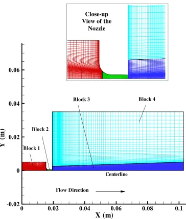
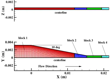
4.2 COMPUTATIONAL GEOMETRY... 75
5 RESULTS AND DISCUSSION... 80
5.1 PURE ETHYLENE INJECTION... 80
5.1.1 Case 1... 80
5.1.2 Case 2... 86
5.1.3 Cases 3 and 4 ... 91
5.2 ETHYLENE/METHANE MIXTURE INJECTION... 105
6 CONCLUSIONS ... 116
7 REFERENCES ... 118
Appendix A: Species Diffusion Velocities and How They Apply to the Governing Equations for Multi-Component, Two-Phase Mixtures... 122
Appendix B: Real Fluid Sound Speed... 127
LIST OF TABLES
Table 2.1: Ethylene and Methane Parameters... 16
Table 2.2: Methods for Calculating Species Viscosities and Thermal Conductivities... 24
Table 5.1: List of Cases for Pure Ethylene Injection... 80
Table 5.2: Mass Flow Rates versus Chamber Pressure (1.0 mm Diameter Nozzle) ... 83
Table 5.3: Predicted and Measured Mass Flow Rates versus Injectant Temperature ... 91
LIST OF FIGURES
Figure 1.1: Pressure Temperature Phase Diagram... 2
Figure 2.1: Ethylene Coexistence Curve ... 17
Figure 2.2: Ethylene Isotherms for Peng-Robinson EOS ... 19
Figure 2.3: Subcritical Isotherm for Ethylene... 20
Figure 2.4: Detailed Subcritical Isotherm for Ethylene ... 22
Figure 2.5: Boiling-Condensation Curve for a Pure Fluid... 32
Figure 2.6: Bubble-Point and Dew-Point Curves for a Binary Mixture ... 33
Figure 3.1: Upwinding Stencil Used for LDFSS Algorithm (ξ direction) ... 67
Figure 4.1: Grid for Axisymmetric Nozzle Simulations... 77
Figure 4.2: Grid for Three-dimensional Nozzle Simulations ... 78
Figure 5.1: Effect of Chamber Pressure on Mach Number ... 81
Figure 5.2: Effect of Chamber Pressure on Liquid Mass Fraction ... 82
Figure 5.3: Ethylene Liquid Mole Fraction Distributions at X/D=112 ... 84
Figure 5.4: Temperature Distributions at X/D = 112... 85
Figure 5.5: Effect of Injectant Temperature on Mach Number ... 89
Figure 5.6: Effect of Injectant Temperature on Liquid Mass Fraction ... 90
Figure 5.7: Effect of Injectant Temperature on Onset of Condensation in Transparent Injector ... 93
Figure 5.8: Centerline Pressure-Density Process Path for Different Injectant Temperatures... 96
Figure 5.9: Effect of Injectant Temperature on Wall Pressure Distributions ... 98
Figure 5.10: Effect of Mesh Refinement on Wall Pressure Distributions at Tinj=281.5 K (Two-Dimensional Calculations)... 99
Figure 5.11: Effect of Injectant Temperature on Centerline Liquid Volume Fraction... 100
Figure 5.12: Pressure Distributions at Tinj = 289.0 K: Homogeneous Equilibrium Model and Nucleation/Growth Model ... 101
Figure 5.13: Liquid Volume Fraction Distributions at Tinj = 289.0 K: Homogeneous Equilibrium Model and Nucleation/Growth Model... 102
Figure 5.14: Contour Plots of Average Droplet Diameter and Droplet Number Density ... 103
Figure 5.15: Average Droplet Diameter and Number Density Distributions (Centerline and Near-wall) ... 104
Figure 5.16: Centerline Pressure-Density Process Path for Ethylene/Methane Mixture Injection for Different Injectant Temperatures ... 106
Figure 5.17: Effect of Injectant Temperature on Onset of Condensation (Liquid Ethylene Mass Fraction): Pure Ethylene Phase Surface Tension and Diffusion ... 108
Figure 5.18: Effect of Injectant Temperature on Onset of Condensation (Liquid Ethylene Mass Fraction): Binary-Mixture Surface Tension and Diffusion ... 109
LIST OF SYMBOLS
Roman Symbols:
±
C split Mach number
k p
C , specific heat at constant pressure for
species k
±
D pressure splitting function
E, ,F G inviscid flux vector in ξ, η, ζ directions v
E , Fv, Gv viscous flux vector in ξ, η, ζ directions
F condensation rate
k
F condensation rate for species k
H total mixture enthalpy per mass
I k
H total mixture enthalpy of phase I for species
per mass
I identity matrix, nucleation rate, phase description
k
I nucleation rate for species k
J Jacobian of a coordinate transformation
Kn Knudson number
M Mach number
w
M mixture molecular weight
k w
M , mixture molecular weight of species k
N particle number density
A
N Avogadro’s number
NL number of components in liquid phase
NS total number of species
NV number of components in vapor phase
±
R L
P, subsonic pressure splitting function
Pr laminar Prandtl number
t
Pr turbulent Prandtl number
[ ]
Pk Parachor of species kR residual vector
S supersaturation ratio
S source term vector
Sc Schmidt number
t
Sc turbulent Schmidt number
T temperature
c
T critical temperature
r
T reduced temperature
U vector of conserved variables
c
U , Vc, Wc contravariant velocities components I
k d
U , ,VdI,k,WdI,k diffusion velocities components of species k in the I phase
V mixture volume
V vector of primitive variables
V grid cell volume
I
V volume of phase I
I
Y volume fraction of phase I
Z compressibility factor
I
Z compressibility factor of phase I
a speed of sound
d average droplet diameter
I
f pure component fugacity of phase I
I k
f fugacity for component k in the I
*
g number of molecules in critical nucleus
h mixture enthalpy per mass
I
h enthalpy of phase I per mass
I k
h enthalpy of phase I for species k per mass
i, j, k indices corresponding to ξ, η, ζ directions
k species, turbulence kinetic energy
b
k Boltzmann’s constant
m total mass
I
m mass in phase I
k
m mass of species k
I k
n total number of moles, particle size distribution I
n number of moles in phase I
k
n number of moles of species k
I k
n number of moles of species k in phase I
p static pressure
c
p critical pressure
r
p reduced pressure
t time
ij
t laminar viscous stress tensor
u, v, w Cartesian velocities in the x, y, z directions i
u Cartesian coordinate in index notation
I i
u Cartesian coordinate in phase I in index notation
I k d
u , , vdI,k, wdI,k Cartesian molecular diffusion velocities for component k in phase I
I k
y mass fraction of species k in phase I
z y
x, , Cartesian coordinates
i
x Cartesian coordinate in index notation
I k
x mole fraction of k in phase I
Greek Symbols:
∆ difference operator
Ω vorticity vector
I
α volume fraction of phase I
ij
δ Kronecker delta
ε turbulent dissipation
ij
λ binary interaction parameter
ν laminar kinematic viscosity
t
ν turbulent kinematic viscosity
µ mixture laminar viscosity
I k
µ mixture laminar viscosity
ξ, η, ζ generalized coordinates
i
ρ total mixture density I
ρ density of phase I
σ fluid surface tension coefficient
ij
τ turbulent stress tensor in index notation
ω specific dissipation rate
I k
ω source term for species k in phase I
Subscripts:
2
1 represents a numerical interface quantity
∞ represents a freestream quantity, infinity
I represents fluid phase
l represents a property in liquid phase
T represents partial derivative with respect to T
c represents critical property
o represents initial condition
r represents reduced thermodynamic variable
p represents partial derivative with respect to p
t represents turbulent property
v represents a property in vapor phase
Superscripts:
± represents positive/negative splitting
I represents fluid phase
IG represents property in ideal gas phase
L, R represents left/right side of cell interface
c represents convective Contribution
k represents chemical species
l represents a property in liquid phase
n represents time level
Accents:
¯ represents a Reynolds averaged mean component,
represents a per mole quantity
' represents a Reynolds fluctuation component
~ represents a Favre averaged mean component,
" represents a Favre fluctuation component
Abbreviations:
BC Boundary Condition
CFD Computational Fluid Dynamics
CFL Courant Friedrichs Levy number
GDE General Dynamic Equation
ILU Incomplete Lower Upper factorization method
LDFSS Low Diffusion Flux Splitting Scheme
MPI Message Passing Interface
TVD Total Variation Diminishing
3D Three-Dimensions
2D Two-Dimensions
Others:
∇ del operator
1
INTRODUCTION
Processes involving supercritical fluids have been explored for different applications such as fluid extraction and chromatography in the chemical industry and fuel injection in the aerospace industry. U.S Air Force high-speed propulsion systems cannot be cooled by conventional techniques due to the temperature limit of current aerospace materials. Regenerative fuel cooling of the airframe and the combustor components is an option that has been explored [5]. Endothermic fuels can be used for regenerative cooling, since they act as a heat sink, undergoing endothermic thermal cracking reactions at very high temperatures. These temperatures are usually much higher than the critical temperature of hydrocarbon fuels. The cooling system is thus responsible for the phase transition of endothermic fuels from a liquid phase to a supercritical-fluid phase.
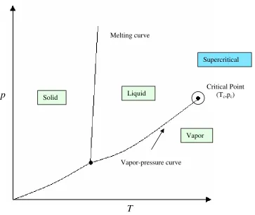
A fluid is defined to be in a supercritical state if its temperature and pressure are above the critical value, where the boundary between liquid and vapor disappear (Figure 1.1). The physical properties of a supercritical fluid are counterintuitive for it exhibits characteristics resembling both liquids and gases in the sense that the fluid has a low viscosity and is highly compressible, like a gas, but is relatively dense and can dissolve a wide range of solid compounds, like a liquid.
favorable for promoting rapid mixing and ignition, as it should be most similar to gas-phase injection. However, condensation (the formation of liquid-fuel droplets) due to fluid expansion may occur under certain injection conditions.
Figure 1.1: Pressure Temperature Phase Diagram
The potential impact of fuel condensation on scramjet combustion is uncertain, and the factors that promote condensate growth should be determined in order to predict its occurrence and to enable its control.
Detailed experimental data on the injection of supercritical ethylene into nitrogen through round-hole (axisymmetric) nozzles were obtained from studies conducted by Wu, et al. [40, 41]. The Wu, et al. database considers parametric variations of the
p
T
Solid Liquid
Melting curve
Vapor
Critical Point (Tc,pc)
Vapor-pressure curve
injectant temperature, chamber temperature, and chamber pressure and presents the effects of these variations on the ethylene jet structure. Under certain conditions, the presence of condensed ethylene liquid phase on the jet structure was indicated by shadowgraph imaging. The onset of this event, most probably driven by homogeneous or heterogeneous nucleation, could not be determined due to difficulties in imaging the internal structure of the round-hole injector used.
Later, Lin, et al. [18] used a transparent, three-dimensional injector configuration with a square exit cross-section to image the onset of condensation. Their numerical model, used to substantiate the experimental results, consists of perfect-gas Navier-Stokes calculations to provide a baseline flowfield for calculating supersaturation and nucleation rates. Onset locations, indicated by a large increase in nucleation rate, were predicted to a reasonable degree, even though supercritical fluid effects were neglected. However, such an approach cannot account for the effects of condensate growth on the flowfield, nor can it give an indication of the amount of condensate present (in terms of a volume or mass fraction).
Lin, et al also considered methane/ethylene mixtures as a more realistic surrogate for cracked JP – class fuels, essentially repeating the Wu, et al. database in the scope of their data collection. More recently, additional data involving pure ethylene injection through round-hole (axisymmetric) nozzles at lower injectant temperatures has been obtained, as have pressure measurements within some of the transparent, three-dimensional nozzles.
mechanisms of supercritical fluid injection for pure ethylene and ethylene/methane mixtures, as well as the onset of condensation upon fluid expansion.
As an initial step, pure ethylene injection into nitrogen through round-hole axisymmetric-nozzles is investigated using the homogeneous equilibrium assumption. Then, pure ethylene injection through a three-dimensional rectangular nozzle is considered using both the homogeneous equilibrium assumption as well as nucleation/growth theory. Finally, binary mixture (ethylene/methane) injection is investigated using nucleation/growth theory.
The fourth code, which solves for the injection of a binary mixture of ethylene and methane, is an extension of the third code applied to a multi-component system.
2
GOVERNING EQUATIONS
2.1
MULTI-COMPONENT
-
MULTI-PHASE DESCRIPTION
All of the cases considered in this study involve two-phase flows which include vapor and liquid phases. When dealing with two-phase flows it is important to introduce new flow parameters, as well as mixing rules which establish relationships between phasic values and bulk values.
Several cases involving the injection of supercritical multi-component mixture have been investigated in this research. In order to implement a multi-component mixture formulation additional terms and relations must be included. In the following sections, mixing rules and physical relations are introduced for phase, multi-component mixtures.
2.1.1 Volume Fraction
The volume fraction is defined as the volume occupied by a particular phase, referenced to the system’s total volume. The vapor volume fraction is given as
V V V V
V v
l v
v
v =
+ =
α (2.1.1)
v v
l l
V V V V V
α
α = = − =1− (2.1.2)
2.1.2 Phasic Mass Fraction and Mole Fraction
The vapor mass fraction, Yv is the ratio of the mass of the vapor phase to the total mass of the system, given as follows
l l v v
v v v
v v v
V V m
m Y
α ρ α ρ
α ρ ρ
ρ
+ =
=
= (2.1.3)
where mv is the mass of the vapor phase, and m is the total mass of the system. In the same manner, the mass fraction of the liquid phase can be written as
v l
l v v
l l l
l l
l Y
V V m
m
Y = −
+ =
=
= 1
α ρ α ρ
α ρ ρ
ρ
(2.1.4)
where ml is the mass of the liquid phase.
2.1.3 Phasic Mixture Properties
The bulk density of the two-phase mixture is defined using Amagat’s law:
(
)
(
p T)
Y T
p Y
l v v
v
, 1 ,
1
ρ ρ
ρ
− +
= (2.1.5)
where Yv is the vapor mass fraction and ρv and ρl are the vapor phase and liquid phase
densities, respectively.
The mixture enthalpy is defined as a mass-fraction weighted average of the vapor
(
p T)
h(
p T)
hh ρvαv v , ρlαl l ,
ρ = + (2.1.6)
or
(
p T)
Yh(
p T)
hY
h= v v , + l l , (2.1.7)
Similarly, the mixture velocity is given as
v i l v i v
i Yu Yu
u = + (2.1.8)
where v i
u is the velocity of gas phase and uil is the velocity of liquid phase in index
notation. If i
l i v
i u u
u = = then the system is in kinematic equilibrium. Kinematic
equilibrium is assumed for all cases considered in this study.
2.1.4 Multi-Component Mass Fraction and Mole Fraction
The multi-component formulation requires the specification of a species mass
fraction which is defined as
∑
= = NS
k k k k
m m Y
1
(2.1.9)
where mk is the species mass within the system. However, the computation of
thermodynamic properties and derivatives are calculated on a phasic basis in which the
species phasic mass and mole fractions are necessary. The mass fraction of species k
relative to the total vapor mass mv and the mole fraction of species k relative to the total
v v k v k
m m
y = ,
v v k v k
n n
x = (2.1.10)
Similarly the mass fraction of species k, relative to the total liquid mass ml and the mole
fraction of species k, relative to the total number of moles within the liquid phase nl are
expressed as
l l k l k
m m
y = ,
l l k l k
n n
x = (2.1.11)
where I k
m , and nkI are the species mass and number of moles for a given phase (I =v or
l
I = ) respectively.
Additional relations are obtained from the fact that all mass and mole fractions
within a phase should add to unity
1
1 1
=
=
∑
∑
= =
NL k
l k NV
k v
k y
y (2.1.12)
1
1 1
=
=
∑
∑
= =
NL k
l k NV
k v
k x
x (2.1.13)
Therefore for a binary mixture the above constraints are reduced to
I I
y
y2 =1− 1 (2.1.14)
I I
x
x2 =1− 1 (2.1.15)
when applying mass conservation to the non-reacting, two-phase, multi-component
(
)
ko l k v vk
vy Y y Y
Y + 1− = , (2.1.16)
where Yv is the ratio of the mass of the vapor phase to the total mass in the system.
2.2
NAVIER-STOKES EQUATIONS
The Navier-Stokes equations are assumed to govern the dynamics of
compressible, multi-phase, multi-component fluids. This set of equations is based on the
independent dynamical laws in continuum mechanics: continuity equation, the
momentum equation and the energy equation. These three equations are the
mathematical statements of three fundamental physical principles respectively:
1. Mass is conserved.
2. Momentum is conserved (Newton’s second Law, F=ma).
3. Energy is conserved.
The non-chemically reacting, compressible Navier-Stokes equations, written in
strong conservation law, vector form for Cartesian coordinates are:
(
)
(
)
(
)
S G G F
F E
E
U v v v
= ∂
− ∂ + ∂
− ∂ + ∂
− ∂ + ∂ ∂
z y
x
t (2.2.1)
where Uis the vector of conservative variables, E, F and G are the inviscid fluxes,
v
E , Fv and Gvare the viscous fluxes, and S is the vector source terms, expressed
− = − − p H w v u Y y Y y Y y Y y Y v l NL l l l v NV v v v ρ ρ ρ ρ ρ ρ ρ ρ ρ ρ 1 1 1 1 M M U , + = − − Hu wu vu p u u u Y u y Y u y Y u y Y u y Y v l NL l l l v NV v v v ρ ρ ρ ρ ρ ρ ρ ρ ρ ρ 2 1 1 1 1 M M E , + = − − Hv wv p v uv v v Y v y Y v y Y v y Y v y Y v l NL l l l v NV v v v ρ ρ ρ ρ ρ ρ ρ ρ ρ ρ 2 1 1 1 1 M M F , + = − − Hw p w vw uw w w Y w y Y w y Y w y Y w y Y v l NL l l l v NV v v v ρ ρ ρ ρ ρ ρ ρ ρ ρ ρ 2 1 1 1 1 M M
G (2.2.2)
− + + − − − − − − =
∑
∑
∑
= = = − − − − y iy i NL k l k d l k l k l NV k v k d v k v k v zy yy xy NV k v k d v k v l NL d l NL l l d l l v NV d v NV v v d v v q t u v H y Y v H y Y t t t v y Y v y Y v y Y v y Y v y Y 1 , 1 , 1 , 1 , 1 1 , 1 1 , 1 1 , 1 0 ρ ρ ρ ρ ρ ρ M M v F (2.2.4) − + + − − − − − − =∑
∑
∑
= = = − − − − z iz i NL k l k d l k l k l NV k v k d v k v k v zz yz xz NV k v k d v k v l NL d l NL l l d l l v NV d v NV v v d v v q t u w H y Y w H y Y t t t w y Y w y Y w y Y w y Y w y Y 1 , 1 , 1 , 1 , 1 1 , 1 1 , 1 1 , 1 0 ρ ρ ρ ρ ρ ρ M M v G , =∑
= − − 0 0 0 0 0 1 1 1 1 1 NV k v k l NL l v NV v ω ω ω ω ω M M S (2.2.5)where vl k d u ,, , vl
k d v ,, , vl
k d
w ,, are diffusion velocities for the vapor or liquid phases of species k
are derived in Appendix A. The number of species in the vapor phase and liquid phase
2.3
SYSTEM CLOSURE: EQUATIONS OF STATE
Closure of the Navier-Stokes equations is achieved by an equation of state
defining the thermodynamic state description of the fluid having the form of
(
l)
NL l
v NV v
x x x x T p
p= ρ, , 1,..., −1, 1,..., −1, and
(
)
l NL l
v NV v
y y y y T h
h= ρ, , 1,..., −1, 1,..., −1, . This investigation implements the ideal-gas equation of state as well as the Peng-Robinson
equation of state.
2.3.1 Ideal Gas Relation
Some of the cases considered in this study involve the injection of ethylene,
initially at supercritical conditions, into a chamber containing pure gaseous nitrogen. For
such cases, the relation between pressure, temperature and density of nitrogen are
obtained from the ideal gas state equation, given as follows:
RT
p=ρ (2.3.1)
where ρ is the molar density ρ/Mw, Mw is the molecular weight, and R is the
universal gas constant.
The ideal gas description for enthalpy and specific heat at constant pressure are
( )
+ +
+ +
+
= k k k k k k
k w k
IG a T a T a T a T a T b
M R T
h 1, 2, 2 3, 3 4, 4 5, 5 1,
,
, 5
1 4
1 3
1 2
1
(2.3.2)
( )
(
4)
, 5 3 , 4 2 , 3 , 2 , 1 , ,
, a a T a T a T a T
M R T
C k k k k k
k w k
IG
p = + + + + (2.3.3)
where coefficients a1,k,...,a5,k and b1,k, for species k, are obtained from McBride, et al.
[23].
2.3.2 Peng-Robinson Equation of State
To account for the thermodynamic behavior of the supercritical fluid, it is
necessary to utilize a generalized state equation, defined by the relations p= p
(
ρ,T)
and(
T)
h
h= ρ, . In this study, the Peng-Robinson equation of state [27] is used for its
simplicity and accuracy when predicting p−ρ−T behavior in both the vapor and liquid regions for hydrocarbons. This equation of state is one of the most commonly used cubic
equations of state, having a similar formulation to the Van der Waals equation. The
Peng-Robinson equation of state for a single-component fluid is given by
(
T)
RT Zp= ρ, ρ (2.3.4)
(
)
( )
( )
(
1 2 2)
1 1 ,
ρ ρ
ρ ρ
ρ
b b RT
T a b T
Z
− + −
−
= (2.3.5)
where ρ is the molar density ρ/Mw, Mw is the molecular weight, and R is the
( )
T a( ) (
Tc α Tr,ω)
a = (2.3.6)
with
( )
c c c
P T R T
a
2 2
45724 . 0
= (2.3.7)
(
)
(
1/2)
2 /
1 , 1 1
r
r T
T ω = +κ −
α (2.3.8)
2
26992 . 0 54226 . 1 37464 .
0 ω ω
κ = + − (2.3.9)
c r
T T
T = (2.3.10)
The constant b is defined as
c c p RT
b=0.07780 (2.3.11)
and other functions used in subsequent developments are as follows:
( )
2 2
T R
p T a
A= (2.3.12)
RT bp
B= (2.3.13)
These parameters are functions of the critical-point temperature Tc and pressure pcof the
Table 2.1: Ethylene and Methane Parameters
Species Tc (K) pc (Mpa) ω
ethylene (C2H4) 282.350 5.0418 0.077523 methane (CH4) 190.564 4.5992 0.011420
The enthalpy of a real fluid can be written as the sum of an ideal gas enthalpy and
a departure function as follows:
(
)
( )
(
)
−
∂ ∂ +
− +
=
∫
∞
v
v w
IG p dv
T p T Z
RT M T h T
h ρ, 1 1 (2.3.14)
For the Peng-Robinson EOS the following enthalpy equation is obtained,
(
)
( )
(
)
( )
( )
(
)
(
)
− +
+ + −
+ − +
=
B Z
B Z
b T a dT
T da T Z
RT M T h T h
w IG
2 1
2 1 ln
2 2 1
1 ,
ρ (2.3.15)
where hIG
( )
T is the ideal gas description discussed previously.2.4
TWO-PHASE FLOWS
All of the cases considered in this study involve two-phase flows which include
vapor and liquid phases. Even though the injectant fluid is initially at a supercritical
state, gas-phase mixing rules are assumed to apply at this fluid phase. This assumption is
adequate as the supercritical fluid expands to gaseous densities upon passing through the
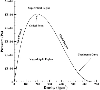
nozzle. The different phase regions of interest in this research are illustrated in Figure
between single phase regions and the two-phase region.
Density (kg/m
3)
P
re
ss
u
re
(P
a
)
0 100 200 300 400 500 600 700
0 1E+06 2E+06 3E+06 4E+06 5E+06 6E+06
Vapor-Liquid Region L
iqu id
R eg
ion
Vap or
Reg ion
Supercritical Region
Critical Point
Coexistence Curve
Figure 2.1: Ethylene Coexistence Curve
2.4.1 Phase Equilibria
To better understand phase transition it is important to explain how the state
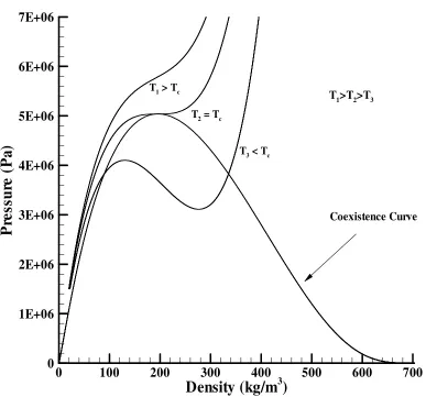
description of the fluid behaves for different thermodynamic conditions. Figure 2.2
indicates the shape of various isotherms for a typical cubic equation of state (the
the supercritical isotherm, where the equation of state description is valid throughout its
extent for it satisfies the criterion for fluid stability which requires that
(
∂p/∂ρ)
>0. TheisothermT2, identified as the critical isotherm, has a single point for which
(
∂p/∂ρ)
=0; and all other points satisfy the condition(
∂p/∂ρ)
>0. Therefore the critical isotherm isalso valid at all locations. The subcritical isotherm T3 is invalid for density values
between spinodal densities located inside the coexistence region where
(
∂p/∂ρ)
<0, butsatisfies the stability condition everywhere else. The loci of these density values for
temperatures between the triple and critical points define liquid and vapor spinodal
curves, dividing the two-phase region into metastable vapor, unstable, and metastable
Density (kg/m
3)
P
re
ss
u
re
(P
a
)
0 100 200 300 400 500 600 700
0 1E+06 2E+06 3E+06 4E+06 5E+06 6E+06 7E+06
Coexistence Curve
T2= Tc
T3< Tc T1> Tc
T1>T2>T3
Density (kg/m
3)
P
re
ss
u
re
(P
a
)
0 100 200 300 400 500 600 700
0 1E+06 2E+06 3E+06 4E+06 5E+06 6E+06
Coexistence Curve
T3< Tc
Spinodal Curve Critical Point
Unstable Region
M eta
sta ble
Vap
or M
etas tab
le L
iqu id
Figure 2.3: Subcritical Isotherm for Ethylene
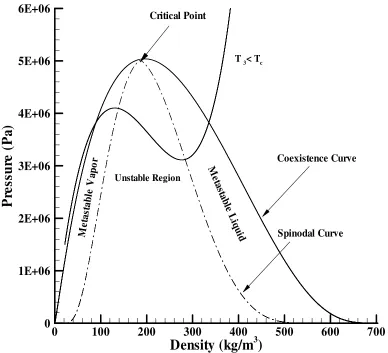
Figure 2.4 displays a more detailed description of the subcritical isotherm T3.
Clearly indicated is the vapor regime, where pressure varies nearly linearly with density,
and the liquid regime, where large pressure changes are required to induce a density
change. For a given pressure and temperature, the solution to the Peng-Robinson
equation of state returns one or three values of the compressibility factor Z, the former
corresponding to the single-phase region (supercritical, liquid or vapor) and the latter
corresponding densities for a pressure within the two-phase region are shown as points
A-C. A and C represent saturated vapor and liquid states, while B is physically
meaningless since it violates the criterion for fluid stability which requires that
(
∂p/∂ρ)
>0. For a particular temperature, the “allowable” two-phase region is boundedby the pressure values at D and E, which are local extrema. At a particular pressure
between the liquid and vapor spinodal points, the system is in equilibrium (for conditions
l v T
T = andpv = pl), with the vapor and liquid Gibbs free energy values being
equal
(
Gv =Gl)
. This pressure is known as the vapor pressure pvap and is calculated as afunction of temperature by iteratively solving the equation
(
v vap)
l(
l vap)
v Z T p f Z T p
f , , = , , (2.4.1)
where the fugacity f is a function of the Gibbs free energy (Gv =Gl ⇒ fv = fl)
(
)
(
)
∫
− =
− =
p IG
dp p RT RT
RT
p T G p T G p f
0
1 1 ,
, ln
ρ (2.4.2)
Using the Peng-Robinson equation of state, the following fugacity relation is obtained
(
)
(
)
(
)
− +
+ + −
− − − =
B Z
B Z
B A B
Z Z
p f
2 1
2 1 ln
2 2 ln
1
ln (2.4.3)
The spinodal pressure and density values (point D and E in Figure 2.4) can be
obtained analytically by solving the quartic equation =0
∂ ∂
T p
ρ , discarding two
The spinodal pressure values bound the actual vapor pressure, and an appropriate linear
combination can be used as an initial guess for the iteration described above.
Density (kg/m
3)
P
re
ss
u
re
(P
a
)
50 100 150 200 250 300 350 400
2.5E+06 3E+06 3.5E+06 4E+06 4.5E+06 5E+06 5.5E+06
T3< Tc
Single-Phase Vapor
Single-Phase Liquid
A B C
D
E
Liquid Spinode
Vapor Spinode
Pvap
Figure 2.4: Detailed Subcritical Isotherm for Ethylene
2.4.2 Mixture properties
When dealing with two-phase flows it is important to introduce new mixing rules
which enable the establishment of relationships between phasic values and bulk values.
are of interest in this study such as mixture viscosity and thermal conductivity. The
two-phase flow mixture viscosity and thermal conductivity are respectively defined as:
l l v vµ α µ
α
µ = + (2.4.4)
l l v vk k
k =α +α (2.4.5)
The gas mixture molecular viscosity is determined by Wilke’s mixing rule [28], and the
thermal conductivity is calculated using Wassijewa’s equation with Mason and Saxena’s
modification [28] defined respectively as follows:
∑
∑
= = = NV k NV l l k v k v k v k v x x 1 1 , φ µ µ (2.4.6)∑
∑
= = = NV k NV j l k v k v k v k v x k x k 1 1 , 065 . 1 φ (2.4.7) where 2 1 , , 4 1 , , 2 1 , 1 8 1 + + = v l w v k w v l w v k w v l v k l k M M M M µ µ φ (2.4.8)The liquid mixture molecular viscosity and thermal conductivity are assumed to be equal
to pure ethylene values for simplicity. The species viscosities and thermal conductivities
Table 2.2: Methods for Calculating Species Viscosities and Thermal Conductivities
Species
ethylene (C2H4) Holland, et al.[16] Holland, et al.[16]
methane (CH4) McBride, et al [23], N/A McBride, et al [23], N/A
nitrogen (N2) Sutherland's Formula Prandtl Number
N/A , 7 . 106 7 . 106 1 . 273 1 . 273 1663 . 0 3 2 2 + + = T T v N
µ , N/A
Pr 2 2 v N v p v N C
k = µ
l k v k µ
µ , l
k v k k k ,
The mixture sound speed, derived in Appendix B, is expressed as
T p T T p T h h h a ρ ρρ ρρ ρ + − = 2 (2.4.9)
where the thermodynamic derivatives of ρp, ρT, hp, and hTare obtained by
differentiating Eqs. (2.6.8 and 2.6.10) with respect to p and T, and are given as
∂ ∂ + ∂ ∂ = p Y p Y l l l v v v p ρ ρ ρ ρ ρ
ρ 2 2 2 (2.4.10)
∂ ∂ + ∂ ∂ = T Y T Y l l l v v v T ρ ρ ρ ρ ρ
ρ 2 2 2 (2.4.11)
p h Y p h Y h l l v v p ∂ ∂ + ∂ ∂ = (2.4.12) T h Y T h Y
h l l
v v T ∂ ∂ + ∂ ∂ = (2.4.13)
The partial derivatives, such as
p l v ∂ ∂ρ , , T l v ∂ ∂ρ , , p hvl ∂
∂ , and
T hvl ∂
Peng-Robinson equation of state.
The Peng-Robinson equation of state (like all cubic equations of state) gives no
useful information in the unstable part of the two-phase region. For densities between
spinodal values, it can be shown that the acoustic eigenvalues are complex, implying that
the Euler system is not hyperbolic in time and that conventional time-marching
procedures for integrating the equation are ill posed. In order to circumvent this problem
two different approaches are used in this study: one is known as the homogeneous
equilibrium two-phase model and the other is a model based on aerosol transport theory.
2.4.3 Phase Transition Models: Homogeneous Equilibrium Model
The homogeneous equilibrium two-phase model replaces the equation of state
description of the two-phase flow by isobars (horizontal lines), ensuring that the
equilibrium phases have the same temperature and pressure (Figure 2.4). The specific
location of the isobars is determined by the assumption of thermodynamic equilibrium
between the vapor and liquid phases whereGv=Gl.
Once density and temperature values are computed from the time-integration
scheme, the following procedure is implemented:
1. For a given temperature, vapor pressure is either calculated by iteratively
solving Eqn. (2.6.1) or obtained from a two-phase coexistence curve. The saturation
densities ρl
( )
T and ρv( )
T and the saturation enthalpies hl( )
T and hv( )
T are thendetermined directly from the equation of state Eqs. (2.6.8) and (2.6.10).
is greater than the critical temperature, then the single-phase description given by the
Peng-Robinson equation is used to calculate pressure and enthalpy.
3. If the fluid density is within the saturation limits and the temperature is below
its critical value, the equation of state is replaced by the homogeneous equilibrium model
given by
( )
T p p = sat⇓
(
)
( )
( )
T( )
T T Tl v
l v
ρ ρ
ρ ρ ρ
α
− − =
,
⇓
(
T)
v(
T)
l ρ, 1 α ρ,α = −
⇓
(
T)
( ) (
T T) (
h T)
( ) (
T T) (
h T)
h ρ, ρv αv ρ, v ρv, ρl αl ρ, l ρl,ρ = +
where the saturation-state enthalpies can be calculated directly from Eq. (2.5.14).
In this formulation, the saturation-state values are strict functions of temperature;
density dependence is introduced through the volume fractions αv,l and latent-heat
effects arise through the change in departure enthalpy between the saturation states. The
above description neglects velocity-slip effects, with the velocity actually solved for
being a mass-weighted average velocity, and thermal equilibrium is assumed. This
system is hyperbolic in character and is similar to the Euler system in structure but admits
such multiphase features as cavitation zones and condensation shocks [6]. Since pressure
two-phase region, density and temperature must be used as the “working” thermodynamic
variables (i.e. the values solved for directly in the CFD code). This formulation applied
to a single component, two-phase mixture allows a simplification of the Navier-Stokes
equations where species and phasic mass conservation equations are eliminated from the
system of equations. Therefore instead of solving NV +NL+4=7 conservation
equations, this method reduces the system to 5 conservation equations (mass=1,
momentum=3, energy=1).
2.4.4 Phase Transition Models: Aerosol Transport Theory
The homogeneous equilibrium model is used due to its simplicity and accuracy in
evaluating flow properties in the two-phase region. However, it does not provide
quantities such as droplet (or bubble) number density, nucleation rate, and average
droplet (or bubble) size. Aerosol transport modeling can be used when those additional
parameters are of interest, due to its ability to simulate the physical mechanisms involved
in a vapor-to-liquid phase transition.
Gas-phase processes, either physical or chemical, can produce a supersaturated
state which then disintegrates by aerosol formation. Physical processes generating
supersaturation include adiabatic expansion and mixing with cool air, among others.
Once condensable species has been formed in the gas phase, the system is in a
nonequilibrium state. The system may attain equilibrium by generation of new particles
(homogeneous nucleation) or by condensation on existing particles (droplets) [13].
Homogeneous nucleation is the process by which condensation nuclei are generated by
formation of new nuclei, when high concentrations of particles (droplets) are present at
low supersaturation.
The mechanism of aerosol formation by gas-to-particle conversion and all
processes influencing the distribution of aerosol properties (aerosol transport) with
respect to particle size are assumed to be modeled by the general dynamic equation
(GDE), which allows for the solution of a droplet size distribution functionn
(
v,r,t)
. Thedroplet size distribution function n
(
v,r,t)
consists of three spatial dimensions, onedimension representing the spectrum of droplet diameters and one temporal dimension.
( )
nt n t
n n D n
t n
coag growth
c
v −∇⋅
∂ ∂ +
∂ ∂ + ∇ ⋅ ∇ = ⋅ ∇ + ∂ ∂
(2.4.14)
The left-hand side of the GDE is comprised of terms modeling temporal and
advective effects upon the droplet size distribution function. The right-hand side consists
of terms representing diffusional growth, gas-to-particle conversion, coagulation, and
sedimentation effects, respectively.
In order to simplify the formulation for the GDE, a locally monodisperse droplet
size distribution (which yields an average droplet size, rather than a size distribution) is
assumed and sedimentation effects are neglected. Two moments of the GDE are of
interest in this study: the droplet number density and the vapor-phase mass fraction.
(
)
coag j j t N I x Nu t N ∂ ∂ + = ∂ ∂ + ∂ ∂ (2.4.15)The nucleation rate I is defined as [11, 17]:
( )
(
)
( )
− = 2 3 2 3 2 / 3 ln 1 3 16 exp 2 S T k v m RT pM I b l e e l v vw π σ
ρ α ρ π σ (2.4.16) where A w e N M
m = is the ethylene molecular mass and
l e l e m v ρ
= is the liquid ethylene
molecular volume. The interfacial tension σ is curve-fitted for ethylene as follows [14]:
− − × = 9 / 11 2 . 133 23 . 23 001 . 0 , 001 . 0 max c c T T T σ (2.4.17)
The limiting value of 0.001 is chosen to avoid extremely high nucleation rates
near the critical point. The supersaturation Sis usually defined as S = p/pvap, however,
since real-fluid effects are significant S is redefined in terms of the ratio of the
vapor-phase fugacity fv to the saturation value fv,eq:
eq v v f f S , = (2.4.18)
The coagulation rate
coag t N ∂ ∂
may be affected by Brownian motion, mean shear,
and Kolmogorov-scale turbulence, among other factors [12]. A comparative study of the
relative effects of the different coagulation mechanisms for a similar problem involving
in Ref. [11]. This study concluded that the largest contribution to the coagulation rate is
due to Kolmogorov-scale turbulence, which increases the collision frequency of the
droplets. The following coagulation rate model of Saffman and Turner [30] for a locally
monodisperse collection of droplets is used in this study:
2 3
2 1 3 16
n d t
N t
N
K turb
coag
− = ∂ ∂ = ∂
∂
τ (2.4.19)
where the Kolmogorov time scale (for a k−ω model) is
υ ω τ
µk
C K
=
1
(2.4.20)
and Cµ
(
=0.09)
is a model constant, k is the turbulence kinetic energy, and ω is the turbulence frequency.The vapor-phase mass fraction expressed in conservative form is written as
(
)
(
)
(
)
NF I g N M x
u Y t
Y
A w j
j v v
+ −
= ∂
∂ + ∂
∂ ρ ρ *
(2.4.21)
where the source term consists of a portion due to the formation of critically-sized nuclei
and a portion due to molecular condensation onto existing nuclei. The number of
molecules which must coalesce in order to form a stable nucleus is given as [17]
( )
( )
3 3
3 / 2 *
ln 1 3
32
=
S T
k v g
b l e
σ π
(2.4.22)
(
,)
2333 . 1 71 . 1 1
1 2
Kn Kn
Kn m
dD
F v veq
e v
+ +
+ −
= π α ρ ρ (2.4.23)
where the Knudsen number is defined as
T k
m d Kn
b e v 2
2 π
ρ µ
= (2.4.24)
and the diffusion coefficient Dis defined by assuming a constant Schmidt number:
v Sc D
ρ µ
= (2.4.25)
The average droplet diameter is determined by the equivalence
3
6d n l
π
α = (2.4.26)
In contrast to the homogeneous equilibrium model, the finite-rate formulation
based on aerosol transport theory requires that the pressure and temperature solved be
“working” thermodynamic variables, allowing the liquid and vapor densities ρv and ρl
to be determined directly from the solution of the cubic equation of state. The finite-rate
formulation assumes kinematic and thermal equilibrium between phases and is strictly
valid in the metastable regions of the vapor dome.
2.5
MULTI-COMPONENT MIXTURES
Several cases involving the injection of supercritical ethylene/methane mixtures
have been investigated in this research, since ethylene/methane mixtures are a more
requires additional terms and relations. In the following sections, multi-component
mixture equilibrium criteria, mixing rules, and physical relations are introduced, and
modifications to equations previously discussed are presented.
2.5.1 Multi-Component Mixture Phase Equilibria
At a given pressure, a pure fluid has a single boiling and condensation
temperature as shown in Figure 2.5. However, boiling and condensation phenomena are
more complex in multi-component mixtures, where at a given pressure and composition,
the boiling and condensation temperatures have different values.
Figure 2.5: Boiling-Condensation Curve for a Pure Fluid
p
T
Solid Liquid
Vapor
Critical Point (Tc,pc)
Consider the vaporization of a binary mixture, for simplicity, composed of 0.5
moles of component 1
( )
lx1 and 0.5 moles of component 2
( )
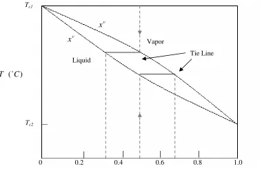
x2l , where Tc1 >Tc2.Figure 2.6: Bubble-Point and Dew-Point Curves for a Binary Mixture
At a given pressure, as the binary liquid is heated, it reaches a temperature at which the
first bubble of vapor is formed, as shown in Figure 2.6. This temperature is known as the
bubble-point temperature of the liquid. The composition of the liquid is essentially
unchanged by its partial vaporization to form one small bubble and is used to determine
the vapor composition of the small bubble (i.e. 2v =0.67
x ). The compositions of the two
coexisting phases at a given pressure are given by the intersection of a horizontal line (i.e.
line of constant temperature) with vapor and liquid curves. This line, which connects the
equilibrium composition in two coexisting phases, is referred to as the tie line. Since the
Tc1
Tc2
Liquid
Vapor v
x v
x
) ( C T o
0 0.2 0.4 0.6 0.8 1.0
Tie Line
vapor is richer in component 2 than the liquid mixture, as boiling proceeds the liquid
mixture will be depleted of component 2. Consequently, as the mixture continues to
vaporize, the liquid will become increasing more dilute in component 2 and its boiling
point will increase.
In the same manner, consider the condensation of the same binary mixture
consisting of 0.5 moles of component 1
( )
vx1 and 0.5 moles of component 2
( )
x2v . As thevapor temperature decreases at a fixed pressure, it reaches a temperature at which the first
droplet of vapor condenses (Figure 2.6). This temperature is known as the dew-point
temperature of the vapor. The composition of the vapor when forming a single small
drop of liquid is essentially unchanged and is used to determine the liquid composition of
the small droplet (i.e. 2l =0.31
x ). Clearly, as the condensation process continues, the
vapor will become increasingly richer in component 2, and the equilibrium condensation
temperature will decrease.
Therefore, the dew point and the bubble point are the equilibrium state of the
mixture at a given pressure and composition (or temperature and composition), similar to
the vaporization pressure in a single component mixture at a given temperature.
In this study the dew point curve is of interest since the conditions investigated for
the ethylene/methane mixture involve phase transitions due to the condensation of the
vapor mixture. The dew point (as well as the equilibrium liquid composition within the
droplet) is calculated as a function of temperature and vapor composition by iteratively