Division VII
MULTI-DIMENSIONAL FRAGILITY ANALYSIS OF A RC BUILDING
WITH COMPONENTS USING RESPONSE SURFACE METHOD
Sreelakshmy Rajan1, Okyay Altay2, Thomas Kubalski1, Luis A Dalguer3, Christoph Butenweg4, and
Sven Klinkel5
1 Research Assistant, Chair of Structural Analysis and Dynamics, RWTH-Aachen University, Germany 2 Chief Engineer, Chair of Structural Analysis and Dynamics, RWTH-Aachen University, Germany 3 Structural Engineer, swissnuclear, Switzerland
4 Professor, SDA-engineering GmbH, Herzogenrath, Germany
5 Professor, Chair of Structural Analysis and Dynamics, RWTH-Aachen University, Germany
ABSTRACT
Conventional fragility curves describe the vulnerability of the main structure under external hazards. However, in complex structures such as nuclear power plants, the safety or the risk depends also on the components associated with a system. The classical fault tree analysis gives an overall view of the failure and the interaction between the components and structure, but it fails to show the cumulative distribution of the failure. As an alternative, Cimellaro et al. suggested a method, which combines the fragility of the structure and the components, by using multidimensional performance limit state functions. This approach gives the possibility of deriving the cumulative fragility taking into account the interaction of different components. Here we use this approach to evaluate seismic vulnerability of a representative electrical building infrastructure, including the components, of a nuclear power plant. A simplified model of the structure, which represents the nonlinear material behavior is modelled using Abaqus©. The input variables considered are the material parameters, boundary conditions and the seismic input. The variability of the seismic input is obtained from selected ground motion time histories of spectrum compatible synthetic accelerograms. Unlike the usual Monte Carlo methods used for the probabilistic analysis of the structure, a response surface method is used. This method reduces the computational effort of the calculations by reducing the required number of samples.
INTRODUCTION
seismic fragilities in NPP using different methods are well explained in Reed and Kennedy (1994), apart from the empirical methods and engineering judgement fragility curves, analytical fragility development using Monte Carlo simulation is included in it. Recently, it is seen in the literature that, fragility curves are developed using numerical simulations, however, most of the analysis are performed on simplified models. Consideration of uncertainty is also crucial in critical structures. More recently Coleman (2014), has shown the nonlinear structure interaction effects on the nuclear facilities considering uncertainty in seismic input. Zentner (2010) developed fragility curve for NPP equipment using non-linear dynamic analysis considering uncertainties in the model as well as uncertainty in the seismic load using Monte Carlo methods.
Monte-Carlo simulations are the commonly used methods for the structural simulations in probabilistic analysis procedures. In order to obtain an accurate failure probability Pf, the number of
samples, n, required to be used at least in the order of 1/ Pf (Gupta and Manohar 2004). The input
variables are combined randomly and deterministic analyses are performed on the structure for each sample. For complex structures, it is computationally impractical to perform Monte Carlo simulation for nonlinear time history response of the structure, even with present day computational capacity. Improved sampling methods like Latin Hypercube sampling, which divides the sampling space into sectors of equal probability of occurrence and selects one realization from each sector, has been used by several researchers for example, Hwang and Huo (1994), Song and Ellingwood (1999), Zentner (2010) etc. Use of surrogate models or meta models for the complex structures are becoming popular in every field. Towashiraporn (2004) used response surface method as a metamodel in combination with Monte Carlo simulation for the fragility analysis of masonry structure. An improved response surface method proposed by Gupta and Manohar (2004) optimizing the response surface in such a way that it includes significant response points which contribute to failure probability.
As a part of the SPRA, the probability of failure of the whole power plant is then determined by the Fault tree analysis which is generally used for the safety and reliability analysis (Paoazoglou 1985). The classical fault tree analysis represents the failure and combination of failure which leads to an undesirable event, assuming that the events are binary and are statistically independent, however complex interactions are not very well represented. As an alternative Rao, et al. (2009) suggested a dynamic fault tree analysis for nuclear power plant incorporating complex interaction by introducing dynamic gates in the fault tree. Other variation of dynamic fault tree was suggested by Čepin and Mavko (2001) which included the time dependent behavior of the nuclear power plant. However, the complex interactions make it difficult to understand and the fault tree analysis is not able to represent the cumulative distribution of failure, like a fragility curve.
The fragility curves developed for the systems should contain, the fragility of the components and the structure and their interaction. A multi-dimensional fragility analysis was suggested by Cimellaro, Reinhorn, et al. (2006), which combines the different failure modes of the components and structures using multidimensional performance limit state function. The method considers multiple limit state parameters, which can be the limit state of the response of component and of structure. They method was applied to a hospital building in California, and the influence of the uncertainty in the performance limit state on the fragility analysis is also illustrated in Cimellaro and Reinhorn (2010). The same approach was utilized by Wang et al for the seismic fragility of highway bridges considering two damage parametrs, column ductitlity and transverse deformation of the abutments.
MULTIDIMENSIONAL FRAGILITY
The seismic fragility describes the conditional probability that the response of the structure or the component exceeds a given limit state under various intensity of seismic excitation. Mathematically, the fragility
P
f(
)
for a particular earthquake intensity Θ can be described as given in Equation 1,
P R s
Pf( ) (1)
Where R is the random variable of the response, for example deformation or acceleration, s is the threshold limit state according to a given degree of damage and Θ is the intensity of seismic excitation such as return period, peak ground acceleration (PGA) or peak ground velocity (PGV). This can be extended for N number of parameters suggested by Cimellaro et al.(2006) and is given in Equation 2,
N i i i N Nf P R s R s R s R s P R s
P 1 3 3 2 2 1 1 .... ) ( (2)
Where Ri is the response parameter related to deformation acceleration, si is the threshold
parameter for a given damage corresponding to the response. In this paper the performance limit state considered are the inter story drift of the reinforced concrete structure and the acceleration of the generator. Therefore, this can be simplified to as shown in Equation 3
s s
f P A A
P ( )
(3)Where Δ is the inter story drift response variable, A is the acceleration response of the generator,
δs, As are the given threshold for inter story drift and acceleration respectively. Therefore, the response in
this curve can be represented using a bell surface (Cimellaro and Reinhorn, et al. 2006) in the acceleration – inter story drift plane. The surface is created with the two variables inter story drift and acceleration responses with a joint probability density function. The maximum responses are assumed to be lognormal distributed
Multidimensional performance limit state
A generalized formulation was suggested by Cimellaro and Reinhorn, et al. (2006), as a tool to consider multiple limit states associated with different response quantities in the same formulation. Different response paremeters like stresses, displacements, velocities, acceleration can be considered to form a combined performance limit state, and hence a unique fragility curve can be plotted for the given system with strcuture and components or the entire facility. The generalized formula (Cimellaro and Reinhorn, et al. 2006) for the multidimensional performance limit state (MPLS) is given as in Equation 4
0 1 .... ) ,.... ( 2 1 2 2 1 1
1
n N n n N N n s R s R s R R R L (4)
Where Ri is the response parameter, si response threshold parameter corresponding to damage and
Ni is the interaction factor which depicts the dependency of the random variable describing the
0 1
0 0
Na
LS LS N
LS LS
A A
(5)
Where δLS0 represents the independent peak inter story drift limit state, ALS0 is the independent
peak acceleration limit state, δLS represents the dependent peak inter story drift limit state, ALS is the
dependent peak acceleration limit state, and Nδ and Na are the interaction factors determining the shape of
the limit state. A further simplified equation is obtained when the interaction factor for inter story drift is assumed to be equal to 1 as given in Equation 6
0 1
0 0
N
LS LS LS
LS
A A
(6)
Where δLS0 ALS0 are independent quantities and are calculated from field data collected or
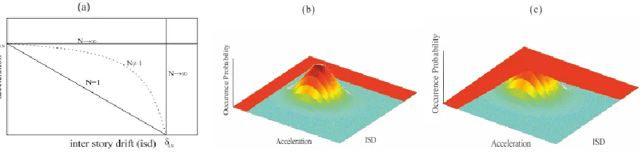
experimental laboratory test. It can be considered as random or deterministic. Limit states can either be linear or nonlinear and is dependent on the value of N. N is determined using the comparison with experimental data and judgement. N takes the real number greater than or equal to 1. When N takes the value 1, the limit state is a line between acceleration and drift which represents the velocity. When N is greater than 1 there is a nonlinear relationship. When acceleration and interstory drift are considered as unrelated, then N tends to infinity and the two parallel lines as shown in the Figure 1 a.
Figure 1 (a) influence of N on the limitstate. (b) Simplified nonlinear model (c)Position of generator
Multidimensional fragility curve development
the performance limit state is calculated by integrating the area under the limit state curve as given by Equation 7
s s
s A A f f Ad dA
P
(7)The domain s is the shaded area in the Figure 1b for the dependent case as shown in Figure 1c and is mathematically represented as in the Equation 8. When the response variables are assumed to be independent, then the probability of exceeding the limit state can be evaluated from the cumulative distribution functions of both the acceleration and the interstory drift responses. In the case when the variables are dependent, then
the number of times
N
f , that the maximum acceleration and the maximumISD exceed a given performance threshold and divide by the total number of trials n related to the respective intensity, so the probability Pf of reaching or exceeding the performance limit state is obtained
as
N
f /n.0 1
0 0
N
LS LS
A A
(
0
,
A
0
)
(8)The procedure is repeated for each intensity and finally the lognormal distribution fragility is plotted using maximum likelihood method or regression analysis.
RESPONSE SURFACE METHOD
Monte Carlo simulations are computationally expensive to get accurate results if complex structures are involved in the calculations with time history analysis. The use of metamodels reduces the computational effort considerably without losing much of the accuracy (Towashiraporn 2004). Response surface methodology (RSM) is one of the most commonly used metamodel, it involves the process of developing functional relationship between random input variables (RIV) and random output variable(ROV), which is the random response of the structure. The main steps involved in the generation of response surface are, design of experiments, choosing a function for the surface representation, fitting the model. The design of experiments is the initial step and several types of experimental designs are available the most commonly used one is the central composite design. Spacing optimized Latin hypercube sampling is used in this paper for the design. Various combinations of input variables are formulated using this method. At these points, structural responses are computed. The relation between the obtained random response and the random input variable are represented using a surface, fitted using polynomial regression. For the polynomial regression model, the function of the response surface is approximated by a polynomial function. The higher the polynomial degree, the more computations are required. To decrease computational effort, the polynomial function is commonly assumed to be of first or second order. Here, second order polynomial is used and is given by the Equation 9,
i j i j
ij i
k
i i i i
k
i
i
x
x
x
x
y
2
1 1
0 (9)
Where y is the ROV, xi; xj are the RIV, β0, βi are the regression coefficients, i represents the
expected change in response y per unit change in xi when all remaining independent variables xj(ji) are
held constant (Myers, et al. 2016). k denotes the number of input variables, and ε the experimental error
evaluated using Monte Carlo method for each PGA, giving the random response corresponding to each peak ground acceleration.
NUMERICAL MODEL AND UNCERTAINTY
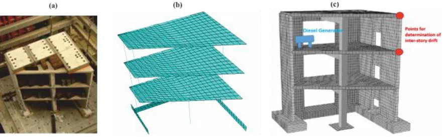
The test structure of the international benchmark project Smart 2013 project (Richard and Chaudat 2014) is considered for the analysis of multidimensional fragility in this study. The test structure is three-storied reinforced concrete structure, and is a 1/4th scaled model of a typical electrical facility of a
nuclear power plant. The technical specification of the strcuture including the general description, seismic inputs, material parameters and fragility analysis recommendations are given in Richard and Chaudat (2014). A simplified model of the test structure is modelled using Abaqus©, representing the material non linearity of the test structure. Figure 2a and 2b shows the geometry and the numerical model of the test structure. The reinforced concrete walls are modelled using the closed section beam elements of Abaqus© with a stringer reinforcement modelled as a box section. The nonlinear material parameters are considered in the reinforced concrete walls and foundation. Concrete damaged palsticity model of Abaqus©, which is a modified Drucker-Prager plasticity is used for the concrete and elastic-perfectly plastic material model for steel. The model is validated for linear properties using the natural frequency and linear time histoy analysis. The nonlinear behavior is validated from the shaking table test results of the benchmark. The model is simplified for the analysis from the previous model presented in Rajan, et al. (2017).
Figure 2 (a) Test structure photo. (b) Simplified nonlinear model (c)Position of generator
Probabilistic Analysis
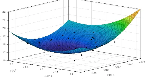
Probabilistic analysis of the system (structure+generator) is carried out using response surface method. A software program Nessus© is used in combination with Abaqus© to obtain the probabilistic response. The design of experiments, is done using spacing-otpimized Latin hypercube sampling. A minimum number of samples recommended in the users manual is chosen, for 4 variables,40 samples are chosen for the response surface method, for each of 30 set of accelerograms. The structural responses are computed at these points in order to obtain the training data to develop a functional relationship between input and output variables. A second degree polynomial function is used to fit the curve to form the response surface. Fitted response surface with two RIV and 1 ROV corresponding to a PGA of 2.5g is shown in Figure 3. It is assumed that the probable response of the structure lies on this surface This function is then evaluated using Monte Carlo for 10000 samples to obtain the optimum response. The random response thus obtained is further used for the multidimensional fragility analysis
Figure 3. Second degree polynomial fitted response surface corresponding to PGA of 2.5g.
DEVELOPMENT OF FRAGILITY CURVES
A reliable assessment of seismic fragility of structures depends mainly on the definition of the level of damage, the failure threshold and seismic intensity measure. The seismic indicator used in this study is the peak ground acceleration. The damage indicator for the structure is defined by maximum interstory drift at point as shown in Figure 2c. Three levels of damage are considered: Light damage (drift = h/400), controlled damage (drift = h/200), and extended damage (drift = h/100), where h is the story height. The generator is assumed to be acceleration sensitive. The acceleration limit state of the generator is a fictitious value. It is calculated based on the natural frequency range of the typical diesel generator of a nuclear power plant. The fragility curve is generally modeled using a lognormal cumulative distribution function, a choice supported by studies in the past in different fields for example Shinozuka et al (2000b). Therefore, the fragility curve is mathematically described as given in Equation 10,
) ln( / )( m
f
A
P (10)
Where Φ is the standard normal probability distribution function, θ is the seismic intensity (PGA in this study), Am is the median capacity expressed in terms of θ, β is the lognormal standard deviation.
m i m i i m i i A z n A z n 1 , ) / ln( 1 ln ) / ln( ln ln max arg ˆ , ˆ
(11)Where zi is the observed probability of collapse out of ni ground motions (samples in the analysis)
with ɵi as seismic intensity, m is the ground motion causing collapse. The fragility curves are plotted
using the maximum likelihood method.
For the multidimensional fragility analysis, in the inelastic behavior the acceleration and the interstory drift are considered as independent of each other and are assumed to be log normally distributed. Therefore, the probability of exceeding the given performance limit state is deducing to equation 12.
sA
A
s
F
A
A
sF
sF
A
A
sF
sP
1
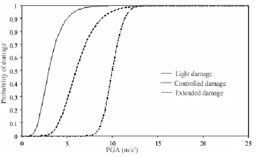
(12)The fragility curves for the system are plotted using maximum likelihood method and is as shown in the Figure 4. The curve depicts the likelihood of damage corresponding to specific damage states with peak ground acceleration. The probability of failure increases with increase in the PGA. The median capacity for light damage is 0.3g and for controlled and extended damage is 0.61g and 1.01g. The maximum deviation is seen in the light damage behavior, equal to 0.4. the total collapse of the structure in the extended damage occurs in all cases occurred at a PGA of 1.63g. The presented fragility curve represents the overall failure of the structure and the component. Therefore, it is capable of representing likelihood of seismic damage is for the system, however, the fragility of each component are not visible individually. The represented fragility curve is only applicable to this test structure with generator.
Figure 4. Fitted fragility curve for the system.
Influence of the interaction factor on the fragility curves
CONCLUSION
As a part of the SPRA, the fragility is a key component of the risk analysis. Generally, in a NPP the fragility curves of various structures and components are used in the fault tree or event tree analysis, which analyses the overall risk of the facility. As an alternative approach to the fault tree, system related fragility curves are proposed to get the fragility curves of the overall system. A method using multidimensional performance limit state (Cimellaro et al. 2006), which can represent different failure types in one formulation, which intern gives a unique fragility curves representing the overall failure of the system including the structure and components is presented here. As an example a test structure with fictitious component is analyzed in the paper. Computationally efficient, Response surface methodology is used instead of the expensive Monte Carlo approach for the probabilistic analysis. The work presented here includes only one component with the structure, however it can be extended to complex systems or components. Expert engineering judgement is required to get the interaction factor N, in the absence of collected data.
ACKNOWLEDGEMENT
The first author also gratefully acknowledges the financial support from BMWi (Bundesministerium fuer Wirtschaft und Energie) and GRS (Gesellschaft fuer Anlagen- und Reaktorsicherheit) gGMBH for the project number 1501503. We would also like to thank the organizers of Smart2013 and the master thesis student Zhenzhi Yu for his contribution.
REFERENCES
Calvi, G. M., R. Pinho, G. Magenes, J. J. Bommer, L. F. Restrepo-Vélez, and H. Crowley. (2006). "Development of seismic vulnerability assessment methodologies over the past 30 years." ISET journal of Earthquake Technology 43: 75-104.
Čepin, Marko, and Borut Mavko. (2002). "A dynamic fault tree." Reliability Engineering & System Safety
(Elsevier) 75: 83-91.
Cimellaro, Gian Paolo, and A. M. Reinhorn. (2010). "Multidimensional performance limit state for hazard fragility functions." Journal of engineering mechanics (American Society of Civil Engineers) 137: 47-60.
Cimellaro, Gian Paolo, Andrei M. Reinhorn, Michel Bruneau, and Avigdor Rutenberg. (2006).
"Multidimensional fragility of structures: formulation and evaluation." Multidisciplinary Center for Earthquake Engineering Research 123.
Coleman, Justin. (2014). "Demonstration of NonLinear Seismic Soil Structure Interaction and
Applicability to New System Fragility Seismic Curves." Tech. rep., INL/EXT-14-33222, Idaho National Laboratory, Idaho Falls, Idaho.
Gupta, Sayan, and C. S. Manohar.(2004). "An improved response surface method for the determination of failure probability and importance measures." Structural Safety (Elsevier) 26: 123-139.
Hwang, Howard H. M., and J. R. Huo. (1994). Generation of hazard-consistent fragility curves for seismic loss estimation studies. National Center for Earthquake Engineering Research. Kennedy, Robert P., C. A. Cornell, R. D. Campbell, S. Kaplan, and H. F. Perla. (1980). "Probabilistic
seismic safety study of an existing nuclear power plant." Nuclear Engineering and Design
(Elsevier) 59: 315-338.
Myers, Raymond H., Douglas C. Montgomery, Anderson-Cook, and M. Christine. (2016). Response surface methodology: process and product optimization using designed experiments. John Wiley & Sons.
Rajan, Sreelaskshmy, Christoph Butenweg, Luis A. Dalguer, Jung Hyun An, and Sven Klinkel. (2017). "Fragility curves for a three-storey reinforced concrete test structure of the international benchmark smart 2013." Proc. of 16th WCEE.
Rao, K. Durga, V. Gopika, V. V. S. Sanyasi Rao, H. S. Kushwaha, Ajit Kumar Verma, and Ajit Srividya. (2009). "Dynamic fault tree analysis using Monte Carlo simulation in probabilistic safety
assessment." Reliability Engineering \& System Safety (Elsevier) 94: 872-883.
Reed, J. W., and R. P. Kennedy. (1994). "Methodologies for developing seismic fragilities." Tech. rep., Electric Power Research Inst., Palo Alto, CA (United States); Benjamin (JR) and Associates, Inc., Mountain View, CA (United States); Structural Mechanics Consulting, Inc., Yorba Linda, CA (United States).
Reed, J., R. Kennedy, D. R. Buttemer, I. M. Idriss, D. P. Moore, T. Barr, K. D. Wooten, J. E. Smith, and others. (1991). "A methodology for assessment of nuclear power plant seismic margin." Tech. rep., Electric Power Research Inst., Palo Alto, CA (United States); Benjamin (JR) and Associates, Inc., Mountain View, CA (United States); Structural Mechanics Consulting, Inc., Yorba Linda, CA (United States); Pickard, Lowe and Garrick, Inc., Newport Beach, CA (United States); California Univ., Davis, CA (United States). Dept. of Civil Engineering; Southern Co. Services, Inc., Birmingham, AL (United States).
Richard, B., and T. Chaudat. (2014). "Presentation of the SMART 2013 International Benchmark."
CEA/DEN Technical Report. DEN/DANS/DM2S/SEMT/EMSI/ST/12-017/H.
Samanta, Pranab K. 1994. Handbook of methods for risk-based analyses of technical specifications. US Nuclear Regulatory Commission Washington, DC.
Shinozuka, Masanobu, Maria Q. Feng, Ho-Kyung Kim, and Sang-Hoon Kim. (2000a). "Nonlinear static procedure for fragility curve development." Journal of engineering mechanics (American Society of Civil Engineers).
Shinozuka, Masanobu, Maria Q. Feng, Jongheon Lee, and Toshihiko Naganuma. (2000b). "Statistical analysis of fragility curves." Journal of Engineering Mechanics (American Society of Civil Engineers) 126: 1224-1231.
Song, Jianlin, and Bruce R. Ellingwood. (1999). "Seismic reliability of special moment steel frames with welded connections: I." Journal of structural engineering (American Society of Civil Engineers) 125: 357-371.
Towashiraporn, Peeranan. (2004). Building seismic fragilities using response surface metamodels. Ph.D. dissertation, Georgia Institute of Technology, Georgia Institute of Technology.
Vesely, William E., Francine F. Goldberg, Norman H. Roberts, and David F. Haasl. (1981). "Fault tree handbook." Tech. rep., DTIC Document.
Wang, Qi’ang, Ziyan Wu, and Shukui Liu. (2012). "Seismic fragility analysis of highway bridges considering multi-dimensional performance limit state." Earthquake Engineering and Engineering Vibration (Springer) 11: 185-193.