Modeling Impact of and Mitigation Measures for Recurring Freeway Bottlenecks

(1)

ABSTRACT

CLARK, ZACHARY THOMAS. Modeling Impact of and Mitigation Measures for Recurring Freeway Bottlenecks. (Under the direction of Dr. Nagui M. Rouphail.)

Recurrent congestion is a continually growing problem on urban freeways. Facility expansions cannot keep pace with the growing vehicle demand. Low-cost mitigation

measures are one way to alleviate the congestion at recurring bottleneck locations. Low-cost measures typically have a life of approximately 10 years and costs ranging from $8,000 to $2.45 million. While benefits have been realized in field applications, only few studies investigated the performance of these measures in terms of added facility capacity.

While micro or macro traffic modeling has long been a tool for planning and

analyzing freeway networks, little has been reported regarding model use for estimating the benefits of low-cost freeway improvements. In this study, the author tested proposed

treatments at two sites using both a macroscopic and microscopic model. Because empirical performance information of these measures is not available, a purely quantitative analysis would not be feasible since confidence in the values reported would be somewhat low.

Current bottleneck identification methods typically either predict breakdown in real-time or analyze detector data off-line. In order to identify bottlenecks from recorded aggregated data in an off-line simulation model, criteria were generated to identify active bottlenecks and analyze the models’ performance in an empirical and qualitative manner.

An assessment of selected available modeling tools is carried out by applying

(2)

from the modeling exercise enabled the evaluation of the models’ ability to simulate the proposed treatments, and the results are used to evaluate the treatment effectiveness on a system-wide basis.

The two most common treatments applied in the case studies are the addition of auxiliary lanes between on and off ramps, and off-ramp facility improvements. Auxiliary lane additions showed reductions of system bottleneck activations in the microsimulation models by 10%, 13%, and 73%. Off-ramp improvements reduced system bottleneck activations in the microsimulation models by 10%, 13% and 32%. In the macrosimulation model, auxiliary lane additions reduced system bottleneck activations by 0%, 33%, and 100% and off-ramp improvements showed a 0% reduction in system bottleneck activations in all instances.

(3)

Modeling Impact of and Mitigation Measures for

Recurring Freeway Bottlenecks

by

Zachary T. Clark

A thesis submitted to the Graduate Faculty of North Carolina State University

in partial fulfillment of the requirements for the Degree of

Master of Science

Civil, Construction, and Environmental Engineering Raleigh, NC

2007 APPROVED BY:

Dr. Joseph E. Hummer Dr. Billy M. Williams

(4)

BIOGRAPHY

Clark, Zachary Thomas

The author was born in Muncie, IN and attended Yorktown High School in nearby Yorktown, IN. Upon graduation in 1997, he attended Indiana University in Bloomington, IN and graduated in 2001 with a Bachelor of Arts in Physics from the College of Arts and Sciences and a minor from the Kelley School of Business.

After graduating from Indiana University, the author was employed by the Steak ‘n Shake Corporation in various management positions in Bloomington, IN. In 2003, he returned to academia to study Civil Engineering at Purdue University in West Lafayette, IN.

(5)

ACKNOWLEDGMENTS

I would like to thank Dr. Nagui M. Rouphail for providing guidance over the past 2 years. His influence and mentoring will always be appreciated. Also, I’d like to thank Dr. Billy M. Williams and Dr. Joseph E. Hummer for participating on my thesis committee and their provided direction.

Finally, I would like to thank the National Cooperative Highway Research Program (NCHRP) and Dr. Alex Skabardonis, PI for their support during the project. Special thanks are also given to Crawford, Murphy & Tilly, Inc. (CMT) and the Wisconsin Department of Transportation (WisDOT) for their help in obtaining needed data and information.

Specifically, I would like to express my gratitude to the following individuals:

• Shawn Leight, Crawford Bunte Brammeier (CBB), for providing data and

information, and his helpfulness and patience in providing answers.

• James Harris, John Shaw, and John Williamson, WisDOT, for their answers to

my many requests and questions.

• Jim Dale, PTV America, for serving as a sounding board during the modeling

stages of the research.

• Wuping Xin, University of Minnesota, for his generosity and efforts in regards

to his software modeling utility.

• Brian Eads, Crawford, Murphy, and Tilly (CMT), for help in understanding the

(6)

LIST OF FIGURES

Figure 1 Bottleneck Analysis Framework...

Figure 2 Milwaukee, WI case study freeway segments...

Figure 3 St. Louis, MO Case Study Freeway Segments...

Figure 4 Interchange of I-44 and I-270...

Figure 5 Plus Lane Operation...

Figure 6 I-894 Segment 18-19 Weaving Section...

Figure 7 St. Louis, MO Segment Speed Profiles...

Figure 8 27th St. Interchange Configurations...

Figure 9 Hale Interchange Configurations...

Figure 10 Westbound I-894 Hale Interchange Ramp...

Figure 11 Initial Proposed Hale Interchange Treatment...

Figure 12 Lincoln Ave. and EB Greenfield Ave. Merge Areas...

Figure 13 Lincoln Ave. and EB Greenfield Ave. Merge Area System Treatment...

Figure 14 NB I-270 Segment 13 Bottleneck Treatments...

Figure 15 SB I-270 Segment 5 Off-Ramp Baseline and Treated Conditions...

(9)

LIST OF TABLES

Table 1 Northbound I-270 Segment 13 (ONR)...

Table 2 Northbound I-270 Segment 10-11 (ONR + LD)...

Table 3 Southbound I-270 Segment 3 (OFR)...

Table 4 Eastbound I-44 Segment 5 (WB)...

Table 5 Westbound I-44 Segment 4 (WC)...

Table 6 Number of Bottleneck Activations/Replications in VISSIM Model – Missouri Site ...

Table 7 Bottleneck Activations in FREEVAL Model – Missouri Site...

Table 8 Number of Bottleneck Activations/Replications in VISSIM Model – Wisconsin Site...

Table 9 Number of Bottleneck Activations in FREEVAL Model – Wisconsin Site...

Table 10 VISSIM and FREEVAL Model Capabilities Summary...

(10)

I. INTRODUCTION

Background

Statistics indicate that congestion delay that is caused by freeway bottlenecks has increased greatly in recent history, and that the top ten freeway bottleneck sites incur approximately 220 million hours of delay per year (1). Bottlenecks have long been

characterized as active when vehicles are discharging from an upstream queue unimpeded by conditions downstream (2, 3). Recurring freeway bottlenecks can arise from many

conditions which include high mainline or merging demand, lane drops, weaving segments, vertical or horizontal curves, and long inclines.

Freeway bottlenecks have received considerable amount of attention because of their impact on safety, economics, and the environment. Large construction projects typically alleviate bottlenecks but are very costly and require large amounts of time for planning and construction. Smaller scale projects have shown to alleviate at least some, if not all, delay caused by recurring bottlenecks. While these measures may not be as broad or long-lasting, they generally have a high benefit-to-cost ratio (4, 5), increase safety (4) and have been shown to reduce driver stress (6).

Literature Review

(11)

Additionally, general driver stress reduction has been studied via surveys (6) and proposed treatments have been reviewed through judgment though not quantitatively (7).

Machemehl et al discuss general guidelines, advantages, and drawbacks of ramp metering. However this study did not provide quantitative results of real-world

implementations. Speed improvements that were observed in a FRESIM analysis are provided in that study (4).

(12)

system-wide treatment can be expected to yield a volume increase in the range of about 2% to 20% and a speed increase on the order of 16% to 30% during the peak analysis period (8).

Another study regarding the use of ramp meters in North America (9) cites the results of several case studies. Of the studies that performed evaluations, the mainline peak period flows increased 2% to 14.3% due to on-ramp metering (9). However, because in these studies the pre-meter conditions were congested, the metering system essentially restored the freeway to pre-breakdown conditions. As seen in other literature (2, 10, 11, 12, 13), this flow increase is comparable to the difference between pre-queue and queue discharge flows. Therefore, this flow increase is what we would expect, and since most macroscopic models do not recognize a decrease in flow upon queue formation, there is no need to model a capacity increase when modeling on-ramp meters.

(13)

During the literature review, no single study was identified regarding the modeling of low-cost bottleneck treatments, the ability of models to properly identify bottlenecks, or the expected or observed performance improvements associated with the modeling of low-cost bottleneck treatments.

Context

The study presented in this paper is a portion of the National Cooperative Highway Research Program’s (NCHRP) project 3-83, “Low-Cost Improvements for Recurring Freeway Bottlenecks”. The objective of the project is to develop a technical guide for identifying existing and future recurring freeway bottlenecks. This technical guide will also provide guidance in determining appropriate low-cost geometric and operational

improvements to mitigate the recurring bottlenecks, and to assess the use of analysis tools in identifying, classifying and evaluating the impact of mitigation measures (14). The focus of this research is on the last features in the guide.

(14)

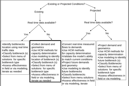
FIGURE 1 Bottleneck analysis framework.

Objective

The objective of the thesis is to assess the abilities of selected modeling tools with respect to (a) identifying recurring freeway bottlenecks (b) to model low-cost bottleneck treatments and (c) how treatments affect the performance of the freeway network. After developing a methodology for identifying recurring freeway bottlenecks in macro and

microsimulation environments, bottleneck treatments were modeled and analyzed. Using the modeling experiences and simulation results of the baseline and treated freeway facilities, the modeling tools were analyzed.

Existing or Projected Conditions?

Existing Projected

Real time data available? Real time data available?

Yes No Yes No

•Identify bottlenecks location using real time traffic data

•Classify bottleneck (s) •Select from menu of solutions for specific bottleneck type •Assess effectiveness in field or via modeling, iterate as needed

•Collect demand and geometrics

•Use HCM methods for capacity determination •Use modeling to identify location of bottleneck (s) •Classify bottleneck (s) •Select from menu of solutions for specific bottleneck type

•Assess effectiveness in field or via modeling, iterate as needed

•Project demand and geometrics

•Use HCM methods for capacity determination •Use modeling to identify future bottleneck (s) •Classify Bottlenecks •Select from menu of solutions for specific bottleneck type

•Assess effectiveness in field or via modeling •Convert real-time measured

flows to demands •Use HCM methods for capacity determination •Validate the model’s ability to match current conditions •Project future demands and geometry

(15)

(16)

II. ORGANIZATION

(17)

III. METHODOLOGY

The objective of this study was to assess and contrast the impact of recurring freeway bottlenecks using macro and micro simulation tools. The dimensions of the evaluation included bottleneck identification, severity and impact of treatments on traffic performance.

In order to formulate criteria for recurring bottlenecks, a quantitative definition of a bottleneck, its severity and recurrence features need to be developed that are appropriate for application in macro and micro simulation environment. The definition used in this study is based on a set of criteria that were formulated from the literature and engineering judgment supplemented by research associated with NCHRP project 3-83.

After gathering network and traffic data for the case study freeway sites that had known recurrent congestion problems, the proposed definition described in the next section was applied to both a macroscopic and microscopic model. A second objective was also to compare how two different analysis tools would identify and classify the bottlenecks in question.

Replications of the baseline (no improvements) model and the post-improvement models were carried out and the frequencies of bottleneck activations at the identified bottleneck locations and treatment effects were compared.

Recurring Bottleneck Identification

(18)

characteristics of the freeway (e.g. steep upgrades), fluctuations in demand, and traffic operations. For this study, the bottleneck needs to appear at the same location at a regular frequency. Additional details are available in NCHRP 3-83 documents (14)

The two selected models do not generate the same outputs from the simulation replications. From the available measures, it is seen that identifying bottlenecks was not particularly difficult.

Common measures are needed to enable comparisons between models. Following the bottleneck activation, the simulation data would generally indicate high densities upstream of the bottleneck, and associated low flows and speeds, while downstream of the bottleneck higher speeds and lower occupancies are expected, unless another bottleneck is active further downstream. Flow density, volume, and speed are measures available in both classes of models. However, thresholds of particular measures should be defined.

It would seem appropriate to associate a vehicle speed reduction of 15-20 mph below the free-flow speed as the speed reduction threshold, but that could vary, depending on the preferences of the state agency. Several studies regarding freeway bottlenecks and

congestion considered defining the vehicle speed at a bottleneck. For example, Chen et al defined it as 40 mph on a freeway with a free-flow speed of 60 mph; a difference of 20 mph (15). As reported in the NCHRP 3-83 Research Plan Proposal, a congestion map from Caltrans District 3 defined a congested segment as one with average speeds lower than 35 mph for 15 minutes or greater. As this information was also based on freeways in California, a free-flow speed of 60 mph is assumed, providing a speed differential of 25 mph (16).

(19)

While thresholds are site specific, they were found to be approximately 19-25 mph below FFS (17). Similarly, Gomes et al characterized heavy congestion (speeds under 40 mph), speeds not reaching full congestion (40 – 55 mph), and free flow (speeds exceeding 55 mph) on a freeway based on speed thresholds in their study (18). In the HCM, a speed drop of 5-21.7 mph occurs between free flow and capacity depending on the free-flow speed (19).

A threshold regarding density and/or demand to capacity ratio should be selected as well. The Federal Highway Administration (FHWA) defines “congested” freeway

conditions as those with a volume to service flow ratio of 0.8 or greater and “severely

congested” conditions with a volume to service flow ratio of 0.95 or greater (20). Bertini and Myton reported a reduction in flow of 3% to 15% upon queue formation. Unfortunately, this study did not include information regarding vehicle speed (12). Cassidy and Bertini reported that the average queue discharge flow rate can be 10% lower than the pre-queue flow rate

(13). Bertini (2), Hall and Agyemang-Duah (11), and Banks (10) all suggest that the queue discharge capacity is on the order of 10% less than the pre-queue flow.

As mentioned earlier, Caltrans District 3 requires that the freeway segment exhibit low speeds for at least 15 minutes to be considered congested (15). The queue features reported by Bertini and Myton reported bottleneck flows ranging in duration from 4 minutes to 22.5 minutes (21). Chen et al defined a bottleneck as sustained if it had at least 25 minutes of active bottleneck activity within 35 consecutive minutes (14). None of these reports required that the bottlenecks be active at any particular weekday frequency.

(20)

al, recurring bottlenecks were identified based on observed data, as opposed to simulation results. Congestion patterns from heavy, typical, and light traffic days as opposed to frequency (18).

In the case of stochastic microsimulation models, if the bottleneck is not activated in a significant proportion of randomly seeded simulation replications, then it is possible that the presence of the bottleneck is merely by chance, because of a confluence of model random number seeds that created a (non-recurring) congested situation. For these reasons a

threshold of 50% was chosen. Therefore, if a bottleneck is active during at least 50% of the simulation replications (modeled in the peak periods), it was judged that the frequency is great enough to warrant its designation as a “recurring” bottleneck location. The rationale for not selecting a higher value is that a microsimulation model is likely to not account for all factors that reduce capacity, including driver distraction, geometric effects such as horizontal curves and sight distance constraints, the effects of heavy vehicle on passenger car headways, etc.

(21)

In summary, and based on a synthesis of the literature review, the following criteria are proposed for identifying recurring bottlenecks in traffic analysis tools.

• Flow downstream of a bottleneck is occurring at a minimum speed that is 85%

of the free flow speed.

• Average vehicle speed upstream of the bottleneck is at least 20 mph below the

free-flow speed.

• A minimum of 5% segment vehicle flow reduction in queue discharge

conditions.

• The three previous criteria sustained for at least one 15-minute analysis period

on the same segment.

• The four previous criteria present for at least 50% of the simulation runs.

(22)

(23)

IV. ANALYSIS TOOLS

Model Selection

At the onset of this study, three simulation models were selected: FREeway

EVALuation (FREEVAL), CORridor SIMulation (CORSIM), and VISSIM as detailed next. FREEVAL is a macrosimulation model based on the Highway Capacity Manual (HCM). It was developed at North Carolina State University (22). Because the HCM freeway segment procedures do not deal with congested freeway conditions (other than reporting a LOS F), FREEVAL uses a speed-flow curve, shock-wave analysis, and some queuing assumptions to model oversaturation (23). FREEVAL uses the abilities of

Microsoft® Excel and Visual Basic programming language to create an uncomplicated macro model of freeway facility operations in a simple spreadsheet format. FREEVAL outputs include segment and facility d/c and v/c, space mean speed, and density contours for undersaturated as well as for congested freeway facilities. FREEVAL reports data for each freeway segment in user defined aggregated time intervals. The data, in conjunction with the speed, density, and volume to capacity graphs generated as part of the output, makes

bottleneck identification, both active and hidden, rather straightforward.

(24)

part of the Traffic Software Integrated System (TSIS) that makes use of TSIS’s graphical user interface (24).

VISSIM was developed at the University of Karlsuhe in Germany in the 1970s (21) and was commercially distributed beginning in 1993 by PTV Transworld AG (25).VISSIM is a microscopic simulation model that is time-step and behavioral based. VISSIM

incorporates the Wiedemann psycho-physical driver behavior model for the traffic

simulator’s car following and lane changing logic. The Wiedemann model makes use of the iterative process of deceleration and acceleration used in car following (26). VISSIM uses links in the simulator however does not use nodes. This non-traditional structure allows users the ability to control traffic operations and vehicle paths (25). VISSIM reports link information, however, due to its microscopic nature will report it in a more detailed manner. Individual vehicle data and the ability to install virtual detectors can provide more precise information on the location of the bottleneck formation. Since FREEVAL lacks this capability, the individual vehicle data feature was not utilized.

As can be seen in the previous paragraphs, even upon selecting models for the study there was quite a difference in the characteristics of the models. It is clear that a comparison of the tools used in this thesis is important and necessary, and will be valuable.

After preliminary modeling efforts with all three models, and discussion among the study team it was decided that only FREEVAL and VISSIM would be further pursued, for several reasons. For one, FHWA support for the CORSIM model is likely to be significantly curtailed in the future. Also, while using CORSIM in the process of compiling the

(25)

file. Third, access to a freeway facility case study was already available in VISSIM format. Finally, it was felt that a single representative micro simulator would be sufficient to carry out one of the study objectives, namely contrasting different classes of tools. At the end, the two models chosen to be used in this study are FREEVAL Plus and VISSIM 4.10.

FREEVAL is based on the Highway Capacity Manual (HCM). Because this manual is widely used in the US and around the world to evaluate freeway systems, it was important for an HCM-based to be represented among the models chosen. While FREEVAL is not a widely known or utilized macroscopic model, it’s ease of use and HCM-based algorithms make it a sensible selection. VISSIM is seeing increased use in the US and abroad for a variety of network analysis problems, and in general is a good representative of modern micro simulation models that practitioners around the country are exposed to. The simulations were replicated on a Dell computer running Microsoft Windows XP Service Pack 2 with an Intel Pentium® 4 3.20GHz processor with 1 GB of RAM.

Model Limitations

Only limitations that pertain to the conduct of this bottleneck identification and analysis study will be discussed in this section. Model limitations outside the scope of this investigation are not reported.

FREEVAL

(26)

Off-Ramp Capacity FREEVAL does not place a capacity on ramps, therefore high off-ramp demands or downstream capacity constraints (such as the presence of a signal) do not propagate congestion on the freeway mainline. This also means that capacity effects of ramp geometry or traffic control at the downstream end of an off-ramp cannot be modeled.

Queue Discharge Rate FREEVAL does not recognize the difference between uninterrupted and queue discharge capacities that has been reported on multiple occasions in the literature

(2, 10, 11, 12, 13). While this does not affect queue formation, it does affect the discharge of queues and therefore affects the duration of the queue and the activation and duration of downstream queues. Because of this limitation, the 3rd criterion in the recurring bottleneck definition cannot be met.

On-Ramp Vertical Queuing FREEVAL uses a simple input-output approach to model ramps and assumes vertical queuing on the on-ramps. Queues on an on-ramp that may spillback onto surface streets are not accounted for, although the expected queue length is computed.

Directional Freeway Facilities FREEVAL cannot model a network of freeways; rather it is limited to individual directional freeway facilities, and

(27)

method to do this is through the use in FREEVAL of the Capacity Adjustment Factor that is applied to alter the HCM capacities.

VISSIM

Temporary Lane Closures It was found during the VISSIM coding process that temporary lane closures and or openings (shoulder use during peak; incidents) cannot be directly modeled in VISSIM 4.10. This is a recognized problem (27, 28) that is indirectly addressed in VISSIM 4.20. While not mentioned in the VISSIM 4.20 User Manual (29) as a way to model temporary lane closures, there is an example of an incident that is provided with the software. The lane closure is created by placing a parking space in the lane that the user desires to be closed, and forcing a vehicle to park in that space at a specified time span. Other methods suggested by PTV (the agent distributing VISSIM), are placing pre-timed signals on the link lane that you wish to open/close or, similar to the aforementioned parking spot example, placing a transit stop at the location of the closure and setting the dwell time equal to the length of the desired closure (28).

The method with the most promise is the VISSIM Lane-Closure Utility which was developed by a doctoral student at the University of Minnesota - Twin Cities. This utility allows the user to close multiple lanes on multiple links, customize closure time for each individual lane, and specify prohibited vehicle classes for each individual lane (27).

(28)

NEMA Controller Emulator The second set of limitations is that fixed-time signals that utilize the National Electrical Manufacturers Association (NEMA) Emulator in VISSIM do not recognize partial seconds in coding cycle lengths. Preliminary analysis suggests that the algorithm it rounds opposite of standard convention. In other words, it rounds down if the partial second is 0.5 or greater, and up if less than 0.5. For example, a cycle length of 4.3 seconds will act as if it is 5 seconds, and a cycle length of 6.8 seconds will act as if it is 6 seconds. This attribute is not of much concern, other than that fixed-time ramp meters cannot be set as fine. No literature has been found citing this issue for either VISSIM or NEMA controllers.

Shoulder Use While Merging The final limitation of the VISSIM model is that vehicles entering the freeway cannot drive on the shoulder if they are unable to merge in the

(29)

V. CASE STUDY SITES

Two case studies were performed in this research: this included one site in

Milwaukee, Wisconsin and another in St. Louis, Missouri. Both sites are in urban areas and have known recurring freeway bottlenecks.

Milwaukee, Wisconsin

The freeway facility selected at this site is a 9.5 mile section of an urban freeway loop, I-894, in southwest Milwaukee, WI. The study site begins at the I-894/I-94 N-S interchange (Mitchell Interchange) and runs west and then north to the I-894 I/I-94 E-W interchange (Zoo Interchange). Site PM peak traffic data were provided by a consultant of WisDOT and a previous study of the site (17). The provider of the information from Hall et al (17) is not known at the time of this draft. Network geometry data were taken from aerial photography. The network and traffic data for this site are from 2003. This is worth noting as changes on the study site have been made since and currently a large nearby freeway interchange (Marquette Interchange) is under construction and is estimated to be affecting the traffic.

The origin-demand matrix of the site is included in the Appendix on pages 85-90. This origin-demand matrix was formulated from a combination of the data from Hall et al

(30)

from the Hall et al study was used to determine the fluctuations in traffic demands across the study period.

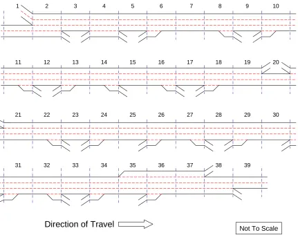
I-894

The directional freeway modeled is composed of 39 freeway segments, which

includes a type C weaving segment, a type A weaving segment, 11 on-ramp merge segments, 2 on-ramp lane add segments, 6 off-ramp diverge segments, and 3 off-ramp lane drop

segments. The remaining 15 segments are basic segments. The segments are shown in Figure 2.

Site Traffic Parameters

(31)

1 2 3 4 5 6 7 8 9

13

11 12 14 15 16 17 18 19 20

10

23

21 22 24 25 26 27 28 29 30

33

31 32 34 35 36 37 38 39

Not To Scale

Direction of Travel

FIGURE 2 Milwaukee, WI case study freeway segments.

Both models were run for twelve 15-minute periods. Periods 4 through 7 represented the peak hour, with a calculated peak hour factor of 0.93.

Because of the lack of detailed speed and volume data at this site, calibration of the model was based on qualitative information gathered from a telephone conversation with a member of WisDOT (30). Default parameters, calibrated parameters from the Missouri (MO) site, and parameters from a site in Pasadena, CA (18) were used in VISSIM

(32)

combination was a result of the MO site non-default parameters focusing on lane changing and the CA site non-default parameters focusing on car following. Additional confidence in the model results can be drawn from the fact that local contacts with individuals familiar with both sites were made. The default parameters, along with the parameters used in the MO site and CA site VISSIM model are located in the Appendix on page 92.

(33)

Calibration of the FREEVAL model was done through adjusting segment type capacities to make them representative of the capacities calibrated in the VISSIM model. After the initial capacity adjustment factors (CAFs) were entered, some fine-tuning was necessary to generate queuing at the appropriate locations.

St. Louis, Missouri

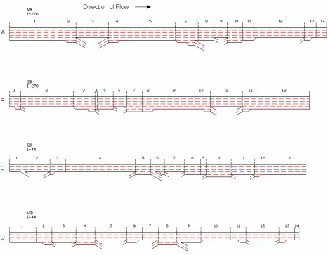
The freeway system chosen as the case study is the interchange of I-270 and I-44 southwest of St. Louis, Missouri and the surrounding area. Network and traffic data were provided by the study consultant to the Missouri Department of Transportation. The traffic origin-demand matrix is located in the Appendix on pages 83-84. This included a calibrated VISSIM data set for the site. Figure 3 displays each freeway direction with segment

numbers. The freeway segments to be analyzed extend approximately 2.75 miles West and South of the interchange and approximately 2 miles North and East of the interchange. There is a collector-distributor road system along the Western segments of I-44.

(34)

Northbound I-270

The Northbound section of I-270 in the study location is approximately 5.58 miles long with 4 mainline lanes. The section is comprised of 14 segments, which includes 3 off-ramp and 3 on-off-ramp segments. The remaining 8 segments are basic freeway segments. None of the ramp influence area overlap and they appear to be operating independent of each other.

Southbound I-270

The Southbound portion of I-270 in the study location is approximately 5.56 miles long with 4 mainline lanes. The section is made up of 13 segments, which includes 4 off-ramp and 2 on-off-ramp segments. The remaining segments are basic freeway segments. As with the northbound direction, none of the ramp influence areas overlap.

Eastbound I-44

(35)

Westbound I-44

The Westbound section of I-44 in the study location is approximately 5.45 miles long with 14 segments. The section begins with 4 mainline lanes and decreases by one lane (corresponding off-ramp) at the 4th segment, which is also a type A weaving segment. There is a type C weaving section at segment 4 and a type B weaving section at segment 8. The weaving segments of the Eastbound and Westbound directions run along side each other.

(36)

FIGURE 4 Interchange of I-44 and I-270.

Segment 8 also contains a speed reduction area (bridge) that covers a majority of the segment. In addition to the two weaving segments, there are 2 off-ramp segments, 2 on-ramp segments, and 8 basic freeway segments. None of the ramp influence areas overlap and are all independent of each other.

Model Calibration

The VISSIM model of this site was originally modeled and calibrated for the

(37)

The existing traffic conditions were based on data collected by CBB and MoDOT. The intersection turning movement volumes were collected by CBB. Existing hourly and historical daily traffic data for I-270 and I-44 and hourly data for all ramp movements were provided by MoDOT (31).

The origin/destination tables were based on traffic counts and weaving observations. These tables were input and modeled as vehicle paths as opposed to turning movement percentages to better reflect actual traffic patterns (31).

Peak hour speed and queue length observations were also performed for model calibration purposes. These were executed using the floating car technique and therefore represent average conditions, and not an 85th percentile speed (31).

The traffic signal timings modeled were based on existing traffic signal timing plans provided by MoDOT (31).

The existing conditions were calibrated so that the modeled volumes on all segments generally fell within 5% or 50 vehicles of actual field volumes. The parameters of the model were adjusted so that the queue lengths and travel speeds reasonably replicated field

conditions. The calibration measures were based on an average of only five random replications of the models (31).

(38)

merge locations, instead of ramp merging and mainline traffic taking turns creating a zipper-like weave, the merging vehicles would be stopped on the acceleration lane waiting for an acceptable gap. This is not what one would expect to observe in the field. In addition to the non-realistic vehicle behavior, this process also caused vehicles to be dropped from the network if they had stayed in the stop position for 60 consecutive seconds.

Site Traffic Parameters

The desired / FFS speed in VISSIM was expressed as a distribution with a median value of 62.3 mph while FREEVAL only allows the input of a single free-flow speed (FFS). This was accounted for, by taking the 50th percentile speed value from the distribution curve in the VISSIM model. This was done for the mainline FFS as well as for the ramp FFS’s. Otherwise, all FREEVAL model default parameters were kept in the baseline runs.

Both models were run for eight 15-minute periods. The first and last two periods were intended to model the shoulder (increase and decrease) demand periods. The third through the sixth periods used vehicle demands representative of the AM peak.

There was only one recurring bottleneck that was communicated to the author based on local site observations, and that bottleneck was determined to be located at the last on-ramp on Northbound I-270 (segment 13 in Figure 3a).

Model Replications

(39)

for the stochasticity in the model results. The number of replications was based on

recommendations in the literature (18, 21, 32) and engineering judgment. The rationale for the single run in FREEVAL is that it is a macro simulation deterministic model, and

(40)

VI. SENSITIVITY ANALYSIS

In order to the test the sensitivity of the simulation software and the previously defined recurring bottleneck definition, a sensitivity analysis was performed.

Origin-destination demands were adjusted to 90, 110, and 120 per cent of the baseline conditions in order to test the sensitivity of the models as well as the previously defined bottleneck criteria. A sensitivity analysis was conducted only at the Missouri site since there was greater

confidence in the level of accuracy in the model calibration at that site.

Simulations

As with the baseline model, each of the adjusted traffic volume models were

replicated 10 times with different random number seeds in VISSIM. Because FREEVAL is a macroscopic model, it was only simulated once per traffic volume adjustment. Five different bottlenecks appeared during the simulations. These are discussed in the following

paragraphs.

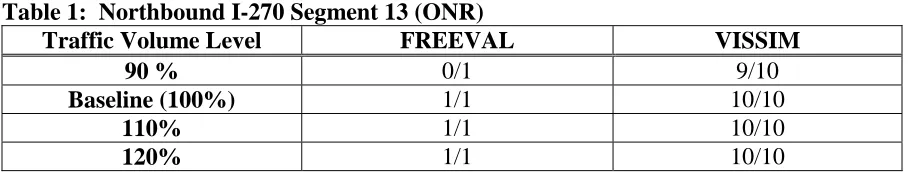
Northbound I-270 Segment 13 (ONR)

(41)

As show in Table 1, even when the traffic volumes are reduced to 90% of the baseline volumes, the bottleneck is activated in 9 of the 10 replications. However, FREEVAL does not predict a bottleneck when the traffic volumes are reduced. The bottleneck is produced in all of the baseline replications, and as would be expected the replications with increased traffic demands.

Table 1: Northbound I-270 Segment 13 (ONR)

Traffic Volume Level FREEVAL VISSIM

90 % 0/1 9/10

Baseline (100%) 1/1 10/10

110% 1/1 10/10

120% 1/1 10/10

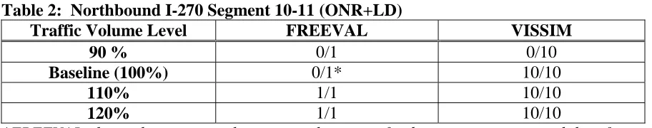
Northbound I-270 Segments 10-11 (ONR+LD)

(42)

Table 2: Northbound I-270 Segment 10-11 (ONR+LD)

90 % 0/1 0/10

Baseline (100%) 0/1* 10/10

110% 1/1 10/10

120% 1/1 10/10

*FREEVAL places the queue on the on-ramp because of a downstream queue and therefore a bottleneck doesn’t show up on the mainline.

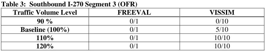
Southbound I-270 Segment 3 (OFR)

Congestion at this segment is actually a byproduct of the bottleneck at the

(43)

Table 3: Southbound I-270 Segment 3 (OFR)

90 % 0/1 0/10

Baseline (100%) 0/1 5/10

110% 0/1 10/10

120% 0/1 10/10

Eastbound I-44 Segment 5 (WB)

This congested location is a type B weave along with a speed reduction zone and a narrowing of lanes, as shown in segment 5 of Figure 3B. A majority of the segment is on a bridge deck. While this segment’s demand does not reach or exceed the capacity as

calculated by the HCM, it does have a high weaving volume (>2,000 vphpl), a moderate volume ratio (vw/V = 0.34), and a moderate weaving ratio (vw2/vw). The volume ratio is not

exceptionally high; however, type B weaving configurations are usually more sensitive to the volume ratio since non-weaving vehicles are more likely to share lanes with weaving

vehicles than in a type A configuration (19).

As can be seen in Table 4 below, VISSIM predicts a bottleneck in 7/10 of the replications with baseline traffic volumes and all of the replications for both the increased traffic volume configurations. FREEVAL only predicts active bottleneck conditions when the traffic volumes are increased to 120% of the baseline conditions.

Table 4: Eastbound I-44 Segment 5 (WB)

90 % 0/1 0/10

Baseline (100%) 0/1 7/10

110% 0/1 10/10

(44)

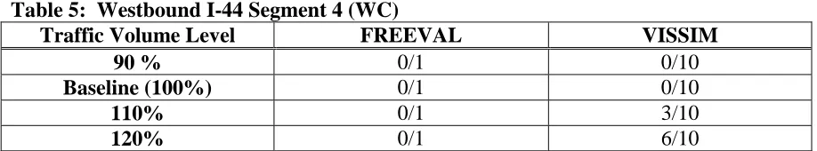
Westbound I-44 Segment 4 (WC)

This section is a type C weaving segment over 2,300’ in length. This weave is shown in segment 4 of Figure 3D. As can be seen in Table 5, active bottleneck conditions are only predicted when volume is increased, and not during the baseline replications. Because a bottleneck does not occur under baseline conditions, treatments will not be modeled at this segment.

Table 5: Westbound I-44 Segment 4 (WC)

90 % 0/1 0/10

Baseline (100%) 0/1 0/10

110% 0/1 3/10

120% 0/1 6/10

Summary

The sensitivity analysis described in this chapter has shown that VISSIM is not highly sensitive to low to moderate changes in traffic volumes. Incremental increases in traffic volume did not create large sways in the frequency of bottleneck activations in the model. This characteristic is reassuring for the modeling of bottleneck treatments. Because of the model’s moderate sensitivity, drastic and unrealistic changes in the network performance are not expected with the introduction of treatments.

The sensitivity analysis results do not seem to reveal much about the FREEVAL model. The segment with the known bottleneck, NB I-270 segment 13, no longer activates a bottleneck when the volume is reduced. However, at the three sites that do not show

(45)

(46)

VII. TREATMENT MODELING METHODS AND RESULTS

Combinations of five types of treatments are modeled and evaluated in the two case studies

• Simple fixed-time ramp metering

• Off-ramp widening

• Auxiliary lane construction

• Restriping and lane-narrowing in conjunction with plus-lane

• Restriping without narrowing lanes.

Ramp Metering

Ramp metering was modeled in VISSIM and FREEVAL using a simple fixed-time strategy that was implemented during the peak period and the following 15-minute period. The capacity of the meter was set to allow the queue created to dissipate before the meter was turned off as well as not spill back onto the surface streets. Meters were located in order to allow appropriate acceleration distance as outlined by the American Association of State Highway and Transportation Officials (AASHTO) Green Book (33). In some instances, where storage was small or the metering was set to favor the freeway, trucks were not required to stop at the meter in the VISSIM model.

(47)

Off-Ramp Widening

In the two instances where off-ramps were widened at the Missouri site, the freeway lanes were converted from a single exiting deceleration lane, to an exiting deceleration lane and a through-exit lane. At the Wisconsin site, the widening was of a freeway-to-freeway ramp which the upstream portion was a freeway split. Instead of 3 lanes splitting to 2 lanes and 1 lane, the 3 lanes split to two 2-lane facilities.

Auxiliary Lane Construction

Auxiliary lane construction was completed by simply adding a full 12-foot lane on the right side of the freeway.

Lane Narrowing and Plus-Lane Addition

(48)

FIGURE 5a Plus lane closed during off-peak period.

FIGURE 5b Plus lane open during peak period.

Restriping was completed by narrowing lanes so that there was room for an additional left-side lane on the existing pavement. Lane restrictions in the VISSIM model kept the trucks from the more narrow left lanes. Reduced speed zones were also created to simulate the expected speed reduction and capacity reduction created by the more narrow lanes. Speeds were reduced in accordance with the HCM lane width adjustment factor for calculating FFS (19).

While there are no examples of this in the United States, through public education, it could become viable option.

Restriping Without Lane Narrowing

(49)

Results Under Baseline Conditions

Using the aforementioned outlined bottleneck criteria, multiple bottlenecks were identified in the models under baseline conditions.

Model Bottlenecks – Wisconsin Site

Segment 1 (Basic) In 1 of the 10 VISSIM replications, bottleneck conditions occur at this location. This segment is essentially a 2-lane freeway connector. The activation appears to be a by-product of a slight slow-down immediately downstream in segment 2, which is a type C weave. Congestion is not predicted in the FREEVAL model, nor is a hidden bottleneck predicted.

While this location does not meet the criteria for a recurring bottleneck, the location will be specially noted since there was an activation in the baseline conditions.

Segment 4 (Type A Weave – 27th St. Interchange) A bottleneck is activated in 7 of 10 VISSIM replications at this segment. The length of the weave is short at 320 feet,

exacerbating the situation as neither of the demands for the ramps are high. A bottleneck was predicted in the FREEVAL model.

(50)

Segment 10 (On-Ramp Merge – Loomis Rd. Interchange) Bottleneck conditions are predicted at this segment in all 10 of the VISSIM replications. The congestion is a result of significant mainline demand and a short taper type on-ramp (approximately 200 feet). The FREEVAL model predicted a bottleneck at this location.

Segment 13 (On-Ramp Merge – 60th St. Interchange) This location does not qualify as a recurring bottleneck by the criteria earlier set forth; however, it does show as a bottleneck in 1 of the 10 VISSIM replications. Because of this section’s location, it creates somewhat of a dilemma. Using the calculated CAF for an on-ramp merge location does not create a hidden bottleneck in FREEVAL, although one would suspect one at this location given the VISSIM results.

The baseline maximum demand to capacity ratio at this location is 0.986 with a corresponding volume to capacity ratio of 0.973, meaning that a hidden bottleneck could be created at this location by reducing the CAF. But since we do not know if the segment is a hidden bottleneck from field verification, it would be irresponsible to force a hidden bottleneck. To remain within the spirit of the study, acting with a lack foresight, a hidden bottleneck will not be forced in FREEVAL at this segment.

(51)

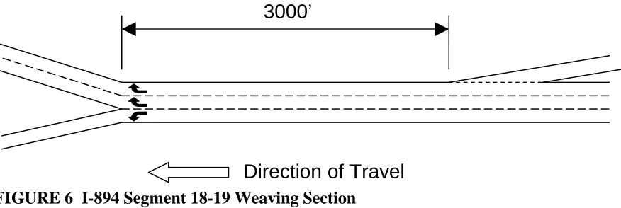
was predicted in the FREEVAL model. Because the distance between ramps is 3,000 feet, it is divided into an on-ramp and off-ramp segment as per HCM standards (19).

FIGURE 6 I-894 Segment 18-19 Weaving Section

Segment 31 (On-Ramp Merge – Lincoln Ave Interchange) This bottleneck is simply created by the merging and mainline demand exceeding the capacity.

This bottleneck was predicted in 7 of 10 VISSIM replications.

In the FREEVAL model, a maximum d/c ratio is predicted above 1, however, the maximum v/c ratio is predicted to be 0.981 and therefore no queue is predicted. The

FREEVAL model does predict a decreased traffic speed (47 mph) and relatively high density (41 vpmpl) at the segment. By FHWA standards, this segment would be considered

“severely congested” (6). Both models, while not necessarily producing similar results, do seem to represent the conditions of the segment as expressed by WisDOT (30).

Segment 34 (On-Ramp Merge – EB Greenfield Ave Interchange) This bottleneck was predicted in 5 of 10 VISSIM replications. Similar to the bottleneck upstream at segment 31,

3000’

(52)

the queuing is created by the demand of the mainline and on-ramp merge is greater than the capacity.

In the FREEVAL model, a maximum d/c ratio is predicted above 1, however, the maximum v/c ratio is predicted to be 0.994 and therefore no queue is predicted. The

FREEVAL model does predict a decreased traffic speed (44 mph) and relatively high density (42 vpmpl) at the segment. By FHWA standards, this segment would be considered

“severely congested” (6). Both models, while not necessarily producing similar results, do seem to represent the conditions of the segment as expressed by WisDOT (30).

Model Bottlenecks – Missouri Site

Northbound I-270 Segment 13 (On-Ramp Merge) This was the original bottleneck communicated by the agency to the author. The bottleneck at this location is caused by the demand from the merging traffic and the mainline traffic exceeding the capacity of the downstream freeway segment. This bottleneck was active in all 10 of the VISSIM replications and in the FREEVAL model. Figure 7a shows the speed profiles from the 2 models at this location. As can be seen in the plot, the bottleneck activations occur at approximately the same time in the simulations. In FREEVAL, and 9 of 10 of the VISSIM replications, the bottleneck becomes active in time period 3. The bottleneck becomes active in 1 of 10 of the VISSIM replications in time period 4. The activation time appears to be longer in VISSIM than in FREEVAL by about one time period (15 minutes).

(53)

hidden by queuing downstream of the section. The rationale here is that the speeds during congestion are lower on segment 10 than they are downstream at segment 13, which is defined as a recurring bottleneck. This can be seen when comparing the speed profiles of the two segments, as seen in Figures 7a and 7b.

This potential bottleneck is similar to that of segment 13’s in that it is possibly caused by high on-ramp and mainline demand. The on-ramp is a two-lane freeway-to-freeway ramp. The congestion is fueled by queuing at downstream segment 13 described above. The congestion is present in all VISSIM replications and the FREEVAL model. Figure 7b shows the speed profiles of the 2 models at this location.

Eastbound I-44 Segment 5 (Type B Weave) The bottleneck at this location is caused by congestion on the off-ramp of the weave. The off-ramp feeds into the on-ramp at segment 10 of NB I-270, which is discussed above. The bottleneck does not appear in FREEVAL

(54)

0 20 40 60 80

1 2 3 4 5 6 7 8

15-Minute Time Period

Av er a g e Vehi c le Spee d ( m ph)

VISSIM Replication Average FREEVAL

FFS

Speed ReductionThreshold

FIGURE 7a Northbound I-270 Segment 13 (On-Ramp Merge) speed profile.

0 20 40 60 80

1 2 3 4 5 6 7 8

FFS

Speed Reduction Threshold

FIGURE 7b Northbound I-270 Segment 10 (On-Ramp Merge) speed profile.

0 20 40 60 80

1 2 3 4 5 6 7 8

FFS

FIGURE 7c Eastbound I-44 Segment 5 (Type B Weave) speed profile.

0 20 40 60 80

1 2 3 4 5 6 7 8

FFS

FIGURE 7d Southbound I-270 Segment 3 (Off-Ramp Diverge) speed profile.

Southbound I-270 Segment 3 (Off-Ramp Diverge) The recurring bottleneck at this location is caused by high off-ramp demand that creates spillback onto the freeway. The bottleneck is active in 5 of 10 of the VISSIM replications. The bottleneck does not activate during the same time period every time. The bottleneck is not predicted in the FREEVAL in the model. It is not activated in the FREEVAL model because FREEVAL does not

recognize off-ramp capacity, as mentioned in the model limitations.

(55)

treatments are modeled at both segment 3 and 5 on Southbound I-270. Figure 7d shows the speed profiles of the 2 models at this segment.

Confirmed Findings The only confirmed bottleneck reported to the research team was on Northbound I-270 segment 13 (Figure 7a). Both FREEVAL and VISSIM predicted bottleneck activations at this location. FREEVAL did not predict bottleneck activations at any other location, whereas VISSIM predicted two other bottleneck location on Southbound I-270 segment 3 (Figure 7b) and Eastbound I-44 segment 5 (Figure 7c). Congestion was reported to us on EB I-44 segment 5 by the modeler but not on SB I-270 segment 3.

The FREEVAL and VISSIM models did not produce the same results regarding bottleneck conditions on the network. This is caused by limitations of the models; most notably the inability for FREEVAL to explicitly model multiple freeway facility interactions and that FREEVAL does not recognize off-ramps as having capacity constraints.

Discussions with the modeler of the VISSIM network confirmed congested

(56)

Results Under Bottleneck Treatment Conditions

Wisconsin Site

Segment 1 (Basic) No treatments were modeled to specifically target this location. However treatments that were performed at segment 4 did have an effect on this location in the

VISSIM model. This is discussed in the following paragraphs.

Segment 4 (Type A Weave – 27th St. Interchange) The baseline conditions of the I-894 interchange with 27th St. can be seen below in Figure 8a. As shown, it is currently a short type A weave. Two treatments were applied at this location.

The first, shown in Figure 8b, is converting the weave to a type B by extending the auxiliary lane, through restriping, past the off-ramp. This was completed in both VISSIM and FREEVAL by adding a lane on the right in order to create 4 lanes in the basic segment immediately downstream of the weaving segment. In order to model the end of the auxiliary lane before the following on-ramp merge, an additional 3-lane segment was inserted.

The second treatment, shown in Figure 8c, is the treatment that has been applied by WisDOT at this location. The treatment involved physically removing the off-ramp of the weave, straightening the downstream on-ramp, lengthening the auxiliary lane through

restriping, and signalizing the surface street intersection. WisDOT did place ramp meters on both of the on-ramps, however those were not modeled in this treatment. This treatment seems to be a more expensive and permanent solution than that shown in Figure 8b.

(57)

immediately downstream at the second on-ramp of the interchange (segment 6). The capacity adjustment factors were not adjusted between treatments. VISSIM did not predict this occurrence.

However VISSIM did predict changes in the bottleneck activations throughout the network, in addition to the one remedied at this location. The changes to the downstream bottlenecks can be mostly attributed to the change in the traffic pattern as well as the increase in arriving demand. One would think that the bottleneck at segment 10 would still meter the downstream traffic and therefore the performance of downstream segments should not be affected, however, the increase in severity (length and duration) of the queuing at this location would create changes in the downstream flows, and therefore the bottleneck activations. The changes in the VISSIM model performance in the upstream congestion in segment 1, is most likely an outcome of the stochasticity of the model as well as the removal of slower traffic downstream.

(58)

FIGURE 8a 27th St. interchange baseline conditions.

FIGURE 8b 27th St. interchange type B weave.

FIGURE 8c 27th St. interchange ramp closure.

320’

R 140’ R 140’

Direction of Travel

Not To Scale

1070’

R 140’ R 140’

Direction of Travel

Not To Scale

720’

R 140’ 45’

R 140’

Direction of Travel

(59)

Segment 10 (On-Ramp Merge – Loomis Rd. Interchange) The treatment that was applied to this bottleneck location was the addition of an auxiliary lane between the Loomis Rd. on-ramp to the downstream off-on-ramp at 60th St. The distance between the two ramps is

approximately 2500’ gore to gore, and would therefore create a type A weave as per HCM definitions (19). This lane addition would be possible through restriping as both the left and right shoulder are approximately 11 feet wide.

The treatment removed the bottleneck activation in all VISSIM replications and in the FREEVAL model. In the VISSIM model, a recurring bottleneck was created at the

downstream on-ramp at 60th St. A bottleneck was active in 6 of 10 replications at the 60th St. on-ramp merge. This bottleneck was not predicted in the FREEVAL model.

In VISSIM this treatment was modeled by adding a lane to the links between the merge and diverge links and connecting them appropriately. In FREEVAL, because the auxiliary lane created a type A weave, the section was changed from an on-ramp merge segment and off-ramp diverge segment to one type A weave segment.

Segment 13 (On-Ramp Merge – 60th Street) As mentioned earlier, this segment

experienced an active bottleneck in 1 out of 10 VISSIM replications and no bottleneck was predicted in the FREEVAL model, and therefore is not a recurring bottleneck. However, a bottleneck does appear in 6 out of the 10 VISSIM replications when the previously described treatment is applied to the Loomis Rd on-ramp merge bottleneck.

(60)

Segments 18-19 (Hale Interchange – Non-HCM Weave) The baseline condition of this section is shown in the top diagram of Figure 9. As can be seen, vehicles that are entering via the on-ramp and wish to exit via the left branch are forced to merge 3 times including the initial merge from the ramp to the mainline. This, in conjunction with the high demand for the left exiting branch, causes a capacity reduction and subsequent bottleneck.

The treatment applied involves widening the exiting left-branch to two-lanes as shown in the bottom diagram of Figure 9. This reduces the number of necessary merges and increases the capacity of the ramp. However, this treatment would require widening the pavement, a bridge deck, and possibly require construction on a bridge overpass and would therefore be a relatively more costly and a long-term solution. The placement of the bridges can be seen in Figure 10.

FIGURE 9 Hale Interchange weave section.

3000’ 500’

Direction of Travel

(61)

FIGURE 10 Westbound I-894 Hale Interchange ramp.

Because the terminal of the downstream end of the ramp widens to two lanes, there would be no need to make changes on the merge area at the ramp’s end. This treatment resulted in only 2 of the 10 VISSIM replications showing a bottleneck, as opposed to 9 of 10 in the baseline conditions. It is worth noting that the treatment resulted in an increase in bottleneck activation downstream at the Lincoln Ave. merge, discussed below, from 6 of 10 to 9 of 10.

An initial treatment was modeled and replicated that widened the ramp from the diverge gore to the viaducts, which is approximately 800’, shown below in Figure 11. The intention was to remove queuing from the downstream freeway and therefore at least provide improvement for the mainline through traffic. However, this was not enough storage space for the queues, so the location still qualified as a recurring bottleneck.

100’ 50m

(62)

800’

Direction of Travel Not To Scale

FIGURE 11 Initial proposed Hale interchange treatment.

Segment 31 (On-Ramp Merge – Lincoln Ave) Figure 11 shows the baseline geometrics of the Lincoln Ave. and Greenfield Ave merge areas. The treatment applied for the Lincoln Ave merge is the auxiliary lane addition between the Lincoln Ave. on-ramp and the downstream off-ramp. The distance between the two ramps is approximately 3150’. This lane addition can be accomplished through restriping without narrowing the lanes.

This treatment removed bottleneck activations at the Lincoln Ave merge in all of the VISSIM replications and the FREEVAL model. The bottleneck downstream at the EB Greenfield Ave. merge was activated 8 of 10 replications with this treatment as opposed to the 6 of 10 replications under baseline conditions. This would be expected as traffic

upstream of the EB Greenfield Ave. merge is able to flow more freely with less obstruction. The treatment also created an active bottleneck in the FREEVAL model at the EB Greenfield Ave. merge.

FIGURE 12 Lincoln Ave. and EB Greenfield Ave. merge areas.

Direction of Travel Not To Scale

(63)

Segment 34 (On-Ramp Merge – EB Greenfield Ave) A schematic diagram of the baseline conditions of this merge area are shown above in Figure 12. As can be seen in the figure, a left-side lane add already exists downstream of the ramp gore. This added lane becomes a freeway-to-freeway ramp in the Zoo interchange, hence the change in lane marking in the diagram. The treatment applied for this bottleneck was to simply extend the downstream lane-add to 1,000’ upstream of the EB Greenfield Ave. on-ramp gore. This treatment could be applied via restriping.

The applied measure resulted in no bottleneck activations in all 10 of the VISSIM replications and in the FREEVAL model.

Treatment Combination Effects No individual treatment targeted at a specific bottleneck location produced model results that significantly improved the modeled system beyond the targeted location. Two system-wide treatments were modeled and are discussed in the following paragraphs.

Hale Interchange – Lincoln Ave. – Greenfield Ave. This treatment combines the individual treatments applied at the Hale Interchange, Lincoln Ave., and Greenfield Ave. bottleneck locations earlier described.

The treatment at the Hale Interchange is exactly as previously described and shown in the bottom diagram of Figure 9.

(64)

a schematic diagram of the baseline set-up. Displayed below in Figure 12 is a schematic diagram of the system treatment that was applied.

Not To Scale

900’ 550’ 1000’ 3150’

Lincoln Ave. EB Greenfield Ave.

Not To Scale

900’ 550’ 1000’ 3150’

FIGURE 13 Lincoln Ave and EB Greenfield merge area system treatment.

The treatment involves changing the Lincoln Ave. on-ramp parallel acceleration lane to an added lane. Upon reaching the downstream off-ramp, instead of dropping the lane, as done when only treating the Lincoln Ave. merge, the lane continues and becomes the far right lane at the EB Greenfield Ave. on-ramp gore by way of lanes shifting. Through existing ample shoulder space and the fact that the ramps are taper type ramps, this can be accomplished through restriping. The benefit of this as opposed to simply combining the individual bottleneck treatments is a reduction in lane changing and a more even and stable flow.

(65)

A weave at segment 3 (27th St interchange) increased its number of bottleneck qualifying replications from 7 to 9 out of 10.

In the FREEVAL model bottlenecks were still predicted at the Hale Interchange and 27th St. weave type A with ramp metering in place. Queuing was not predicted at any of the other previously discussed locations.

Missouri Site

Northbound I-270 Segment 13 (On-Ramp Merge) The treatment applied at this bottleneck location was the addition of an auxiliary lane extending to the following downstream off ramp. The original condition is shown in Figure 14A with the auxiliary lane treatment shown in Figure 14B. Because the ramps are approximately 3,600’ apart, adding the auxiliary lane would not create a weaving segment by Highway Capacity Manual standards. Therefore, adding the downstream off-ramp to the model is not necessary. While the construction of an additional lane is perhaps not a low-cost solution, it will provide a comparison of conditions if a lane was simply added.

(66)

1000’

10’ 10’ 11’ 11’ 11’

A

B

C

Dir

e

c

tio

n

of

T

rav

el

Not To Scale

FIGURE 14 NB I-270 Segment 13 bottleneck treatments.

(67)

the recurring bottleneck on segment 5 of EB I-44. In VISSIM, this treatment was carried out by narrowing the lanes, adding speed reduction zones based on the lane adjustment factor in the HCM, and adding pre-timed signals in the added left lane spaced approximately 25’ apart. The plus lane treatment did remove the bottleneck in the FREEVAL model.

Northbound I-270 Segments 10 (On-Ramp Merge) The addition of the auxiliary ramp downstream and the restriping and plus-lane treatment at segment 13 on-ramp merge

removed the bottleneck at this location in FREEVAL and all VISSIM replications. Also, the system ramp metering treatment removed the bottleneck at this location in all VISSIM replications. Even though no specific treatments were modeled at this segment, two treatments initially intended to primarily remove the downstream bottleneck, removed the congestion on this segment.

Because this bottleneck did not activate once the downstream queue was removed, this segment was not by definition a recurring bottleneck under baseline conditions. Had the bottleneck at this segment still been present after the downstream queue was removed, that would have indicated this was a hidden bottleneck.

(68)

off-ramp lane drop, analysis shows that the treatment did not alleviate the bottleneck at segment 3, as it was activated in 6 of 10 VISSIM replications.

A B

D

irection of T

rave

l

Not To Scale

FIGURE 15 SB I-270 Segment 5 off-ramp baseline and treated conditions.

(69)

the ramp is approximately 30’ wide, it might be possible to restripe and achieve the same results without additional construction.

A

B

Direct

ion of T

rave

l

Not To Scale

FIGURE 16 SB I-270 segment 3 off-ramp baseline and treated conditions.

(70)

It is worth noting, as shown in Table 6, that the number of replications with bottleneck activations at this segment increases for treatments that were not applied at this segment in the VISSIM model. This phenomenon simply demonstrates the effect of model stochasticity on the results, even though the same random seeds were used for each

scenario’s ten replications.

Eastbound I-44 Segment 5 (Weave Type B) System-wide ramp metering (Meters at Northbound I-270 segments 2 and 13, Eastbound I-44 segment 5 On-Ramp, and Westbound segment 5 Off-Ramp as shown in Figure 4) did not completely remove the bottleneck at this location. A bottleneck was still active at this segment in 4 of 10 VISSIM model replications. Since it is only active in 40% of the replications, it does not qualify as a recurring bottleneck location.

The congestion at this segment was shown to be completely alleviated with the addition of an auxiliary lane and a plus lane at segment 13 of NB I-270 described above. There were no active bottlenecks at this location in any replications with either treatment.

Similar to SB I-270 segment 5, and as shown in Table 6, the number of replications with bottleneck activations at this segment changes for treatments that should have had no effect on the traffic conditions at this location in the VISSIM model.