Design, Development and Analysis of Advanced Airboat Propeller by Using Bamboo Composite Fibre Material

(1)

IJEDR1404016

International Journal of Engineering Development and Research (www.ijedr.org)

3475

Design, Development and Analysis of Advanced

Airboat Propeller by Using Bamboo Composite Fibre

Material

1

Shaik Azmatullah Rahaman,

2

Dr. S. Selvarajan,

3

Y.N.V.Santosh Kumar

1

Post Graduate Student, 2Chief scientist, 3Assistant Professor 3Head Of the Department

1,3_{Department of Aerospace Engineering, Nimra Institute of Science and Technology, Ibrahimpatnam-521 456, AP, India.}

2_{Council of Scientific and Industrial Research - National Aerospace Laboratories, Bangalore-560 037, India.}

________________________________________________________________________________________________________

Abstract - The objective of this paper was design, development and analysis of propeller by using a bamboo composite fibre material with contra rotating advance airboat propellers, airboat propeller shows characteristics of its non-aviation usage. The design of a propeller is broad, flattened blade and squared-off tips because the aerodynamic favors a high drag that is useful for slowing an airboat. A simple method of predicting the performance of a propeller is the use of Blade Element Theory. In this method the propeller is divided into a number of independent sections along the length. At each section a force balance is applied involving 2D section lift and drag with the thrust and torque produced by the section. At the same time a balance of axial and angular momentum is applied. This produces a set of nonlinear equations that can be solved by iteration for each blade section. The resulting values of section thrust and torque can be summed to predict the overall performance of the propeller.

Key Words - Propeller, Computer Aided Three-Dimensional Interactive Application, Computational Fluid Dynamics Blade Element Theory

________________________________________________________________________________________________________

Nomenclature-B = number of propeller blades a = Speed of sound, [m/s] C= Chord [m]

CD= Drag coefficient

CL = Lift coefficient

CP =Power coefficient

CQ = Torque coefficient

CT = Thrust coefficient

J = advance ratio parameter KT = thrust coefficient,

N = revolutions per minute [RPM] n = revolutions per second [rps] Q = torque [in-lb]

r = propeller radius [m] T = thrust [lb]

ρ = density [slugs/ft3] 𝜼p = propeller efficiency

I.INTRODUCTION

A. Airboat

The first airboat was built in 1905 in Nova Scotia, Canada. An airboat also known as a fan-boat is a flat-bottom vessel and powered by either an aircraft or automotive engine it is very popular means of transportation, parts of the Indian river, the y are used for fishing, hunting and eco-tourism, and in other marshy or shallow areas where a standard inboard or outboard engine with a submerged propeller would be impractical.

(2)

IJEDR1404016

3476

Figure 1: Airboat

B. Propeller

A propeller is a type of fan that transmits power by converting rotational motion into thrust. A pressure difference is produced between the forward and rear surfaces of the airfoil-shaped blade, and a fluid (such as air or water) is accelerated behind the blade. Propellers on airboats are operated at speeds below the maximum tip speed. In general the maximum tip speed of a propeller is around 890 feet per second.

C. Bamboo Fibres

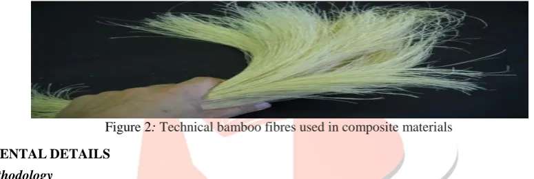
It is to develop a natural fibre composite with high mechanical properties and to present it as a new natural and renewable option to reinforce both thermoplastic and thermoset matrices, which fits into the requirements (properties, availability and cost) established in the field of reinforcements for composites.

Figure 2: Technical bamboo fibres used in composite materials

II.EXPERIMENTALDETAILS

A. Design Methodology

The propeller blade is one of the most complicated parts in the propulsion system, It would take direct effect on the structural intensity，vibration，reliability and life-span. There are many engine failures caused by the problems of shroud design. The coordinate points of NACA 4412 can be generated by using CATIA V5R19 software. Airfoil coordinates are taken from the journal papers, as shown in fig. 3. The blade information data had given in table-1

Figure 3: NACA 4412 airfoil Figure 4: Propeller Blade In part design

Table 1: Blade Information Propeller diameter [D][m] 1.2192 Density [kg/m3] 1.225 Relative Velocity[m/s] 25 Number of Blades [Nb] 2

(3)

IJEDR1404016

3477

A propeller blade can be subdivided into 10 cross section, each cross section is look like an airfoil (as shown in table-2) a discrete number of sections. For each section the flow can be analysed independently if the assumption is made that for each there are only axial and angular velocity components and that the induced flow input from other sections is negligible.

Table 2: Blade geometry

S.NO AIRFOIL SECTION X (mm) Y (mm) CHORD LINE (mm) DISTANCE FOR THE HUB (mm)

1 B-B 88.9 54.7878 104.4194 50.8

2 C-C 89.662 50.292 102.7938 112.776

3 D-D 97.028 37.846 104.14 175.006

4 E-E 97.536 28.956 101.7524 236.982

5 F-F 96.012 22.86 98.7044 299.212

6 G-G 94.234 18.542 96.0374 361.188

7 H-H 90.17 15.24 91.44 423.418

8 I-I 82.804 12.7 83.7692 485.394

9 J-J 73.152 10.16 73.8632 547.624

10 K-K 60.452 7.366 60.9092 609.6

B. Computational Fluid Dynamics

Computational fluid dynamics, usually abbreviated as CFD, is a branch of fluid mechanics that uses numerical methods and algorithms to solve and analyze problems that involve fluid flows. Computers are used to perform the calculations required to simulate the interaction of liquids and gases with surfaces defined by boundary conditions.

C. Geometric Modelling

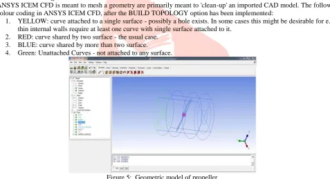
ANSYS ICEM CFD is meant to mesh a geometry are primarily meant to 'clean-up' an imported CAD model. The following is the colour coding in ANSYS ICEM CFD, after the BUILD TOPOLOGY option has been implemented:

1. YELLOW: curve attached to a single surface - possibly a hole exists. In some cases this might be desirable for e.g., thin internal walls require at least one curve with single surface attached to it.

2. RED: curve shared by two surface - the usual case. 3. BLUE: curve shared by more than two surface.

4. Green: Unattached Curves - not attached to any surface.

Figure 5: Geometric model of propeller D. Boundary Conditions

The continuum was chosen as fluid and the properties of air were assigned to it. A moving reference frame is assigned to fluid with a rotational velocity (2800rpm to 10000 rpm). The wall forming the propeller blade and hub were assigned a relative rotational velocity of zero with respect to adjacent cell zone. A uniform velocity 25 m/sec was prescribed at inlet. At outlet outflow boundary condition was set. The far boundary (far field) was taken as inviscid wall and assigned an absolute rotational velocity of zero. Fig. 6 shows the boundary conditions imposed on the propeller domain.

(4)

IJEDR1404016

3478

III.RESULTS

The performance of propeller is conventionally represented in terms of non-dimensional coefficients, i.e.  thrust coefficient (KT),

 torque coefficient (KQ) ,

 advance coefficients (J).

 propeller efficiency and

or

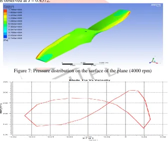
A complete computational solution for the flow was obtained using Cfx software. The software also estimated thrust and torque from the computational solutions for different rotational speeds (rps) of the propeller. These were expressed in terms of KT & KQ. The estimated thrust and torques are shown in Table 4. Comparison of estimated non-dimensional coefficients and efficiency (η) against experimental predictions, as obtained from literature, are shown in Table-4. The comparison of predicted KT & KQ with numerical data. It shows that KT and KQ coefficients are decreasing with increasing of advance coefficients (J). Maximum efficiency is observed at J = 0.4572.

Figure 7: Pressure distribution on the surface of the plane (4000 rpm)

(5)

IJEDR1404016

3479

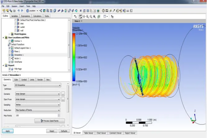
Figure 8: Path Lines at downstream of propeller (4000 rpm)

Graph 2: Turbulence Kinetic Energy Distribution over the Blade (4000 Rpm)

Table 3: Total Torque around Blade for Different Rpm

Torque x [Q] [Nm] Torque y [Q] [Nm] Torque z [Q] [Nm] Total Torque[Q] [Nm]

37.4013 0.0322883 37.43609594 86.0583

42.6654 0.0368846 42.70091128 131.889

48.1873 0.0413366 48.22515778 180.394

80.1976 0.0679474 80.26428537 464.598

121.378 0.071195 121.5276527 819.128

131.025 0.0638003 131.2040801 898.59

136.042 0.057171 136.2384426 939.178

141.214 0.0489022 141.4285843 980.765

151.979 0.027282 152.2354243 1065.6

175.335 -0.0426409 175.6934025 1242.21

244.806 -0.35163 245.4511029 1706.68

412.286 -0.39711 412.5606849 2508.83

577.206 -0.29 577.3081396 3138.77

736.354 -0.430704 736.4126557 3765.25

886.274 -0.637828 886.3183913 4304.88

(6)

IJEDR1404016

3480

Table 4: Efficiency Calculation for the Blade for Different Rpm

Propeller rotational Speed [ṅ][rpm] Propeller rotational Speed [ṅ][rps] Thrust[T] [N] Total Torque[Q] [Nm] Thrust Coefficient [KT] Torque Coefficient [KQ] Advance Ratio [J] Propeller Efficiency [ƞProp]

2800 46.66667 1.61338 86.0583 0.0146 0.005209 0.653143 29.15%

2900 48.33333 1.74072 131.889 0.020858 0.005539 0.630621 37.81%

3000 50 1.91004 180.394 0.026659 0.005846 0.6096 44.27%

3500 58.33333 3.27045 464.598 0.050444 0.007148 0.522514 58.72%

4000 66.66667 6.0288 819.128 0.068092 0.008286 0.4572 59.83%

4100 68.33333 6.85244 898.59 0.071099 0.008515 0.446049 59.31%

4150 69.16667 7.31329 939.178 0.07253 0.00863 0.440675 58.98%

4200 70 7.7877 980.765 0.073949 0.008746 0.435429 58.62%

4300 71.66667 8.83217 1065.6 0.076652 0.008982 0.425302 57.80%

4500 75 11.2164 1242.21 0.08159 0.009465 0.4064 55.78%

5000 83.33333 17.7804 1706.68 0.090799 0.010711 0.36576 49.37%

6000 100 15.0471 2508.83 0.092691 0.012502 0.3048 35.98%

7000 116.6667 10.8553 3138.77 0.085198 0.012853 0.261257 27.58%

8000 133.3333 9.28443 3765.25 0.078249 0.012553 0.2286 22.69%

9000 150 8.84765 4304.88 0.070688 0.011937 0.2032 19.16%

10000 166.6667 12.9785 4920.22 0.065441 0.011159 0.18288 17.08%

Graph 3: RPM Vs Efficiency

Graph 4: RPM Vs Thrust 0

0.2 0.4 0.6 0.8

0 2000 4000 6000 8000 10000 12000

Efficiency

RPM

RPM Vs Efficiency

Rpm Vs Efficiency

0 5 10 15 20

0 2000 4000 6000 8000 10000 12000

T H R U S T N RPM

RPM Vs Thrust

(7)

IJEDR1404016

3481

Graph 5: RPM Vs Torque

IV.CONCLUSIONS

From the above analysis and graphs it can be clearly seen that the maximum propeller efficiency is 59.8% (60%). However the maximum efficiency occurs at 4000 rpm itself. This is a lower rpm for a boat application. However, the efficiency has to increase to get better efficiency.

The effort has been taken to optimize the propeller design to get higher efficiency and higher design rpms. The design characteristics has been studied and has been concluded that by changing the overall span of the propeller may increase the thrust. Since the span has been constrained for a particular air boat.

V.ACKNOWLEDGEMENTS

The authors are thankful to The Director and all the scientists of Council of Scientific and Industrial Research - National Aerospace Laboratories, Bangalore for supporting the research work. Also like to thank all the supporting staff of Nimra Institute of Science and Technology, Vijayawada.

VI.REFERENCES

[1] Optimization of an Airboat Design-Adam P. Leppek by Western Michigan University

[2] Blade element and momentum theory. Helis.com. [Online] [Cited: 15 April 2010.] http://www.helis.com/howflies/bet.php. [3] ANSYS: Introduction to FLUENT. [PDF document] s.l. : ANSYS, Inc. Proprietary, 2009.Salvatore, F., Testa, C., Ianniello,

S. and Pereira, F. 2006. Theoretical modeling of unsteady cavitation and induced noise, INSEAN, Italian Ship Model Basin, Rome, Italy, Sixth International Symposium on Cavitation, CAV2006, Wageningen, The Netherlands.

[4] A Three-Equation Eddy-Viscosity Model for Reynolds-Averaged Navier-Stokes Simulations of Transitional Flow,” ASME Trans. J. Fluids Eng, 130(12), pp. 121401.1–121401.14.

[5] ANDERSOJN.D, . Jr. (1990) Modern Compressible Flow: With Historical Perspective, 2nd Edition (McGraw-Hill)

[6] E.N. Jacobs, K.E. Ward, & R.M. Pinkerton. NACA Report No. 460, "The characteristics of 78 related airfoil sections from tests in the variable-density wind tunnel". NACA, 1933.

[7] Aerospaceweb.org | Ask Us - NACA Airfoil Series

[8] Bansal AK, Zoolagud SS. Bamboo composites: material of the future. J Bamboo Rattan 2002 [9] Murphy RJ, Alvin KL. Variation in fibre wall structure in bamboo. IAWA Bull 1992

[10] Wong KJ, Zahi S, Low KO, Lim CC. Fracture characterization of short bamboo fibre reinforced polyester composites. Mater Des 2010

[11] Das M, Chakraborty D. Role of mercerization of the bamboo strips on the impact properties and morphology of unidirectional bamboo strips–Novolac composites. Polym Compos 2007

[12] Okubo K, Fujii T, Yamamoto Y. Development of bamboo-based polymer composites

[13] Ghoshal AK. Bamboo fibre reinforced polypropylene composites and their mechanical, thermal, and morphological properties. 2011

[14] Joshi SV, Drzal LT, Mohanty AK, Arora S. Are natural fibre composites environmentally superior to glass fibre reinforced composites 2004

[15] Reddy GR, Reddy HK. Flexural and compressive properties of bamboo and glass fibre-reinforced epoxy hybrid composites. J Reinf Plast Compos 2010;

[16] “1991 Yamaha FZ FZR600 Dyno Dynamometer Result Graph. N.d. Photograph. Drag TimesWeb. 25 Mar 2012. <www.dragtimes.com/1991-Yamaha-FZ-Dyno-Results- Graphs-8173.html>.

[17] http://www.aerodyndesign.com/PROP_10/PROP_10.htm 0

200 400 600 800 1000 1200

0 2000 4000 6000 8000 10000 12000

Torque

RPM