Cost of Living Indices
Ian A. Crawford
November 1997
ProQuest Number: U644131
All rights reserved
INFORMATION TO ALL USERS
The quality of this reproduction is dependent upon the quality of the copy submitted. In the unlikely event that the author did not send a complete manuscript and there are missing pages, these will be noted. Also, if material had to be removed,
a note will indicate the deletion.
uest.
ProQuest U644131
Published by ProQuest LLC(2016). Copyright of the Dissertation is held by the Author. All rights reserved.
This work is protected against unauthorized copying under Title 17, United States Code. Microform Edition © ProQuest LLC.
ProQuest LLC
789 East Eisenhower Parkway P.O. Box 1346
C on ten ts
A b stra ct 7
A ck n ow led gem en ts 11
D ecla ra tio n 13
1 In tro d u ctio n 15
1.1 Existence ... 18
1.1.1 Revealed Preference T e s t s ...20
1.2 Uniqueness ...24
1.3 Construction: Estimation and A p p ro x im atio n ...27
1.3.1 E stim ation... 27
1.3.2 A p p ro x im atio n ... 28
1.4 Problems of Measurement and B i a s ... 31
1.4.1 Survey B ia s e s ... 32
1.4.2 Economic Biases ...34
1.5 Conclusion and Sum m aries... 40
2 D isa g g reg a tin g th e C ost o f L iving Index; A n E m pirical In v e stig a tio n for th e U .K . 1979 to 1992 46 2.1 In tro d u ctio n ... 46
2.2 Household Cost of Living I n d i c e s ... 48
2.2.1 Non-Homotheticity and Differential Indices...48
2.2.2 Choosing an I n d e x ... 52
2.2.3 D a t a ... 55
2.3 Non-Housing M e asu res... 58
2.4 Indirect T a x a tio n ... 65
2.5 H o u s in g ...68
2.5.1 The Mortgage Interest A p p r o a c h ... 74
2.5.2 The User Cost A pproach... 78
3 R ev ea led P r eferen ce T ests and N onparam etric E n gel C urves 87
3.1 In tro d u ctio n ... 87
3.2 Individual D ata and Revealed Preference...91
3.2.1 Revealed Preference and Observed D e m an d s... 91
3.2.2 Choosing a Path for Comparison Points ... 92
3.2.3 Nonparametric R egression... 102
3.2.4 Pointwise Inference for Pairwise Comparisons ... 103
3.2.5 Quality Change, Conditional Demands, Separability and CARP ... 105
3.3 Preference H eterogeneity... I l l 3.4 An Empirical Investigation on Repeated Cross-Sections . . . . 114
3.4.1 D a t a ...114
3.4.2 Semi-parametric Estimation and Demographics . . . .1 1 4 3.4.3 Endogeneity and Semi-parametric Correction... 115
3.4.4 Estimated Engel Curves and N orm ality...117
3.4.5 R e su lts... 118
3.5 Summary and Conclusion ... 123
4 R ev ea led P referen ce M eth od s for B ou n d in g True C ost o f Liv ing Ind ices 141 4.1 In tro d u ctio n ...141
4.2 True Indices and A pproxim ations... 143
4.3 Bounds from Revealed Preference... 147
4.3.1 Classical B o u n d s ... 147
4.3.2 Improving the B o u n d s ... 151
4.4 Local Average Demands and Local Average W elfare...158
4.5 R e su lts... 160
4.5.1 Non-Rejecting Sub-Periods... 161
4.5.2 Cost of Living bounds and Approximations...162
4.5.3 Substitution Bias and Non-Homotheticity ...165
4.6 Summary and C o n c lu s io n ...168
5 N e w G o o d s B ia s in C ost o f Living Indices: A R ev ea led P ref eren ce A p p roach 170 5.1 In tro d u ctio n ... 170
5.2 The Problem of New G o o d s ...172
5.3 A Parametric Approach ...177
5.4 A Revealed Preference A p p r o a c h ... 177
5.4.1 Improving the B o u n d s ... 182
5.5 An Empirical Application: Valuing the National Lottery . . . 189
L ist o f Tables
2.1 The post-war experience in the UK, 1939-1980’s... 51 2.2 Grouped average non-housing budget shares, FES, 1978 and
1992... 62
3.1 Number of rejections of G ARP, by size of test...120 3.2 Number of rejections of G ARP, by size of test, virtual price of
tobacco... 122 3.3 Commodity Group: Definitions...125 3.4 Total Nominal Household Expenditure: Annual descriptive
statistics... 126 3.5 First stage equation...132 3.6 Endogeneity-corrected Regression, goods 1 to 5, 1974 to 1983. 133 3.7 Endogeneity-corrected Regression, goods 6 to 11, 1974 to 1983. 134 3.8 Endogeneity-corrected Regression, goods 1 to 5, 1984 to 1993. 135 3.9 Endogeneity-corrected Regression, goods 6 to 11, 1984 to 1993. 136 3.10 Endogeneity-corrected Regression, goods 12 to 16, 1974 to 1983.137 3.11 Endogeneity-corrected Regression, goods 17 to 22, 1974 to 1983.138 3.12 Endogeneity-corrected Regression, goods 12 to 16, 1984 to 1993.139 3.13 Endogeneity-corrected Regression, goods 17 to 22, 1984 to 1993.140
4.1 Continuous periods of convergence... 161 4.2 CARP bounds and approximations to the 1974-based true index. 162
L ist o f F igu res
1.1 Spending growth and the power of revealed preference tests. . 23
2.1 The Engel curve for domestic energy, FES, 1992 ... 50 2.2 The relative price of domestic fuel, UK, 1978-92... 50 2.3 Inflation rates, by income group, per cent, 1979-92 ... 58 2.4 Difference in inflation rates, by income group, percentage points,
1979-92... 59 2.5 The relative price of some necessities: food, electricity, cloth
ing, 1978-92 ... 60 2.6 The relative price of some luxuries: catering, entertainment
and services, 1978-92... 61 2.7 Difference in inflation rates, by employment status, percentage
points, 1979-92... 63 2.8 Differences in inflation rates for the 1st income decile,with and
without taxes, percentage points, 1979-92... 67 2.9 Differences in inflation rates for the 10th income decile,with
and without taxes, percentage points, 1979-92... 67 2.10 Nominal user cost of shelter, £ per annum, 1978-93... 71 2.11 Shelter costs; rents, mortgage payments, RPI method and the
User Cost, 1978-93... 72 2.12 Inflation with and without housing costs; all households, RPI
measure, per cent, 1979-92... 75 2.13 Inflation rates by tenure, RPI measure, per cent, 1979-92. . . . 75 2.14 Difference in inflation rates, by income group, RPI measure,
percentage points, 1979-92... 76 2.15 Difference in inflation rates, by head of household’s data-of-
birth cohort, percentage points, 1979-92... 78 2.16 Inflation rates, with and without housing, all households, user
cost and RPI shelter costs measures, per cent, 1979-92... 79 2.17 Differences in inflation rates, by tenure, user cost measure,
2.18 Differences in inflation rates, by income group, percentage
points, 1979-92... 81
2.19 Difference in inflation rates, by head of household’s data-of- birth cohort, percentage points, 1979-92... 82
3.1 The PMP comparison - low initial total expenditure...95
3.2 The PM P comparison - high initial total expenditure... 96
3.3 The SMP path ... 98
3.4 A non-SMP path with identical preference ordering... 99
3.5 An SMP path with a rejection... 100
3.6 An alternative SMP p a t h ... 101
3.7 The Engel curve for B r e a d ... 118
3.8 The Engel curve for E n te rta in m e n t... 118
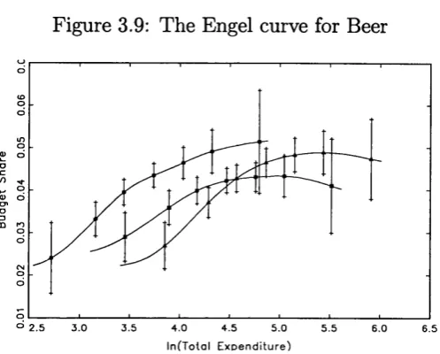
3.9 The Engel curve for B e e r... 119
3.10 The median SMP quantity path for tobacco... 122
3.11 The 1st quartile MP quantity path for tobacco... 123
4.1 Classical bounds, one observation...149
4.2 Classical bound, two observations... 150
4.3 GABP-improved lower bound, two observations...151
4.4 G ARP- improved upper and lower bounds, two observations. . 152
4.5 GARP-improved bounds...155
4.6 Classical and G ARP bounds on the 1974-based true index. . . 163
4.7 Paasche, Laspeyres and Fisher’s indices and G ARP bounds. . 164 4.8 The Tornqvist index and GARP bounds...164
4.9 Bounds in 1981, by total expenditure quantile, (1974=1000) . 166 4.10 Percentage substitution bias, by total expenditure quantile ( 1 9 8 1 ) ...167
4.11 Maximum percentage substitution bias in inflation rates, by total expenditure q u a n ti l e ...168
5.1 Bounding the virtual price, a two good, two period example. . 180
5.2 A negative virtual price, a two good, two period example. . . . 182
5.3 Bounding the virtual price, a two good, four period example. 183 5.4 The improved bound, a two good, two period example...186
A b stra ct
The correct measurement of changes in the cost of living is important for
many reasons. Indeed, the many uses to which measures of inflation are put
make it difficult to overstate the importance of obtaining an accurate value.
For example, the rate of inflation is important in wage settlements, the in
dexation of social security benefits, estimates of macroeconomic growth rates
and, generally, all economic analyses which require knowledge of real, rather
than nominal, magnitudes. Unfortunately, whilst a true cost of living index
(which is defined as the ratio of the minimum cost of reaching a given level of
economic welfare under alternative sets of prices) is a fairly straightforward
theoretical concept, in practice its validity and the way it should be imple
mented are much less clear. The overall theme of this thesis is that of trying
to address some of the fundamental issues which cost of living indices face
without assuming either the existence or the form of the preferences which
might underlie an index.
Chapter 1 introduces some of the ideas which appear later and describes
some of the central issues. It defines the idea of a true cost of living index
and discusses methods of determining whether a given dataset is compatible
with the existence of a single, unique cost of living index constructed from
it. The two main approaches to measuring cost of living indices; approxi
measurement, some of which arise when approximations are used, and some
of which are encountered whatever the method adopted for computing the
index. It concludes with summaries of the material contained in the following
chapters.
Chapter 2 is an empirical investigation into the question of uniqueness;
the extent to which different types of households have experienced differential
changes in their cost of living in the period 1979 to 1992. It also considers
the question of the influences which indirect tax changes over the period
may have had, and looks at the effects which the method used to calculate
housing costs has on the resulting indices. Overall, the fall in the relative
price of necessities and the corresponding increase in the price of luxuries
over the period studied, and the difference in expenditure patterns between
rich and poor households have meant that the cost of living has increased
slightly faster for richer households than it has for poorer households. The
progressive nature of indirect tax reforms between 1979 and 1992 is shown
to have contributed to this effect. The use of a user cost of housing approach
to measuring shelter costs gives evidence of widely different inflation rates
by date of birth cohorts as older cohorts reap large capital gains on housing
over the period.
While Chapter 2 takes the idea of existence for granted. Chapter 3 con
siders the issue in more detail. The basic question asked is; is the empirical
evidence consistent with the existence of a cost of living index ? So far this
has proved difficult to answer. This is for two reasons. Firstly, many studies,
particularly those which use microeconomic data, have found that paramet
ric econometric models reject the hypothesis of utihty maximisation or cost
minimisation. But whether this is due to econometric misspecihcation or
circumstances the hypothesis under test is a joint one; namely th at (a) the
consumer has rational preferences and (b) that the functional form of these
preferences is consistent with the econometric model. We have no easy way
of telhng whether a rejection is due to (a), or to (b) or to both (a) and (b).
Secondly, while revealed preference tests present the possibility of avoiding
this simultaneity (since they don’t require functional form assumptions) the
data used to carry out the tests often lack the power to reject the theory.
This is because income growth often swamps relative price movements so
th at budget hyperplanes may not cross. If budget planes do not cross then it
is impossible to reject the revealed preference conditions for rational choice.
A further problem with revealed preference tests is that, so far, they have
lacked a stochastic framework within which to judge the seriousness of any
rejections. This chapter suggests a method which uses nonparametric En
gel curves to simultaneously improve the power of revealed preference tests,
and to make the problem amenable to statistical testing. It also looks at a
method which, in the event of rejections, can be used to allow for changes in
the quahty of goods or equivalently changes in preferences for a particular
good over the period of the data.
Chapter 4 concerns the question of the construction of true cost of hving
indices. Estimating true indices is computationally difficult and, as described
above, the results may conflict with the theory. A literature has grown up
around the issue of how to compute exact or approximate cost of living in
dices without estimating full, integrable demand systems. This approach
uses a mixture of first and second order approximations, and indices which
correspond exactly to certain forms for preferences but which are also simple
to implement. If we do not wish to make functional assumptions, however,
of limitations in the data. This chapter presents a method of using revealed
preference restrictions in conjunction with nonparametric Engel curves to im
prove the bounds available without the need for assumptions on functional
forms. The improvement is shown to be quite significant. This is used to ex
amine the question of substitution bias, to revisit the question of uniqueness
and to look at the question of whether substitution bias, which affects price
indices with fixed quantity weights, varies with total expenditure.
Chapter 5 is concerned with another source of bias; specifically with the
problem of new goods bias in price indices. This is an area in which func
tional form m atters a great deal. A cost of living index needs to include the
price of the new good for the period before the one in which it first existed
in order to account properly for the welfare effects of its introduction. Func
tional form m atters a great deal here as in order to do this the main method
has been to use parametric demand systems to extrapolate the demand curve
to the point at which demand becomes zero. The results of such an exercise
are fikely to be heavily dependent on functional form. This Chapter de
scribes a nonparametric method which uses revealed preference restrictions
to place a lower bounds on the virtual price of a new good without the need
for functional form assumptions. This is the lowest bound consistent with
the (partly testable) maintained hypothesis that the data are, on average,
A ck n ow led gem en ts
I would particularly like to thank Laura Blow, Richard Blundell and Martin
Browning for their help. Chapter 2 is joint work with Richard Blundell and
Martin Browning. Part of the theoretical work in chapter 4 is joint work with
Laura Blow. I would also hke to thank my supervisors Ian Preston and David
Ulph, and all of my colleagues at the Institute for Fiscal Studies, past and
present. In particular I would like to thank James Banks. Part finance for this
thesis has been provided by the E.S.R.C. Centre for the Microeconometric
Analysis of Fiscal Pohcy at I.F.S. and is gratefully acknowledged. The Family
Expenditure Survey data used in this thesis was made available by the O.N.S.
through the E.S.R.C. Data Archive. The author is solely responsible for any
D ecla ra tio n
No part of this thesis has previously been presented to any University for
any degree.
C h apter 1
In tro d u ctio n
This thesis is about aspects of cost of hving indices: their existence, their
uniqueness, their construction and problems encountered in the course of
their measurement. The calculation and use of index numbers is essential
to most aspects of social accounting, since without the aggregation of the
great mass of information on quantities and prices which they perform, raw
economic data would be difficult to comprehend. Further, the many uses
to which measures of the rate of change of the cost of living (inflation) are
put, make it difficult to overstate the importance of obtaining an accurate
value. For example, the rate of inffation is important in wage settlements,
the indexation of social security benefits, estimates of macroeconomic growth
rates and, generally, all economic analyses which require knowledge of real,
rather than nominal, magnitudes. Practicality is thus a prime concern in
much of the literature on cost of living indices; as Deaton (1981) points out,
cost of living indices combine “side-by-side some of the most difficult and
abstruse theory with the most immediately practical issues of everyday mea
surement”^. Afriat (1977) questions whether, in most practical situations,
this abstruse theory and its associated paraphernalia of utility functions and
cost functions really contributes very much of any use. He argues that “util
ity functions give service in theoretical discussions where they contribute
structure which is an essential part of the m atter”^. In fact they often confer
exactly such an essential structure. Stone (1956), for example, suggested
three reasons why the utility-based approach is useful in defining and con
structing indices:
“First, they give content to such concepts as real consumption
which might otherwise be vague and obscure; second they bring
out fundamental difficulties in establishing empirical correlates to
concepts such as real consumption and so help to show what can
and what cannot usefully be attempted in the present state of
knowledge; finally they show the circumstances in which partic
ular empirical correlates ... are likely to provide a good or a bad
approximation to the concepts of the theory.”^
These are precisely the concerns of this thesis. This chapter introduces
some of the material which will appear later. The plan is as follows. Section
1.1 concerns the question of existence. It defines the idea of a true cost of
hving index, and discusses methods of determining whether a given dataset
is compatible with the existence of a cost of living index constructed from it.
It turns out that testing a dataset for consistency with the existence of a cost
of hving index is, at least in principle, a relatively straightforward matter. In
practice, however, it may often be the case that the nature of the available
data makes informative application of the theory difficult.
If we are unable to reject the hypothesis that a suitable index exists us
ing, say, data on the average demands of a sample of households, the matter
^Afriat (1977), p. 3.
of how we can compute the index remains. The first issue is whether the
data are consistent with the existence of a unique index which is identical for
all households, or whether different indices should be calculated for different
households. Generally speaking it has been found th at cost of living indices
vary with household characteristics and incomes and that a single index is
therefore not universally applicable. This is considered in section 1.2. If this
can be resolved, then the question of actually computing the index or in
dices arises. This is discussed in section 1.3 which summarises the two main
approaches to measuring cost of living indices; approximation and full para
metric estimation. In practice, parametric estimation may be both difficult
and unreliable, and nonparametric bounds or approximations are often used.
Section 1.4 discusses problems of measurement, some of which arise when
approximations are used, and some of which are encountered whatever the
method adopted for computing the index - even full parametric estimation.
Section 1.5 concludes the introduction and summarises the contents of the
next four chapters which seek to make a contribution in all of these areas.
Chapter 2 is an empirical investigation into the pattern and extent of
variations in the rate of change of the cost of hving between different types
of households and households with different incomes. Chapter 3 presents
a framework which improves the method whereby a finite dataset can be
tested for consistency with the neoclassical model of consumer choice. It
also looks at the issue of changes in quality or tastes, which can both lead
to a rejection of the neo-classical model. Chapter 4 uses the techniques
applied in Chapter 3 to develop a method of recovering two-sided bounds
to true cost of living indices. It also revisits the question of differences in
indices by total expenditure and provides an assessment of how well popular
this chapter provides. Chapter 5 looks at another problem common to both
price indices and true cost of living indices: the arrival of new goods. The
normal parametric method of estimating the virtual price of a new good
(for inclusion in an index) is both computationally expensive and heavily
dependent upon a maintained hypothesis concerning the functional form of
preferences. Chapter 5 presents a method of bounding this virtual price
which is both computationally straightforward and does away with the need
for functional form assumptions.
1.1
E xisten ce
Change can only be recognised through reference to some standard which
persists unchanged. In the case of the cost of living index the standard is
a given level of economic welfare. The cost of living index measures the
changing cost of reaching this standard as prices change. Traditionally in
economics, the standard of living is measured by the welfare derived from
consumption^. The concept of the true cost of living index was introduced by
Koniis (1924) and is defined as the minimum cost of achieving the reference
welfare level ur when prices are pt, relative to the minimum cost of achieving the same welfare with prices pg. In notation this is written as
= (1.1)
c{Ps,Ur)
where c{pt,UR) is the consumer’s cost or expenditure function evaluated at the period t price vector P( and the reference welfare level u r. The cost
function is central to the whole area of cost of living indices and is defined
by
c {p ,u r) = m i n q { p ' q : n ( q ) > u r} (1.2 )
where the utility function u (q) is usually assumed to be a real value function
with the three properties (i) continuity, (ii) increasingness and (iii) quasi
concavity. The reference welfare level can be chosen more or less arbitrarily,
however Us and Ut are often popular and obvious choices since, by the assump tion of cost minimising behaviour on the part of consumers, the cost functions
evaluated at (pt, Ut) and (p^, Us) are directly observable: c (pf, Ut) = pjqt and
c{ps,Us) = p^qg. Note that as the index depends upon utility, comparing
two indices with two different reference welfare levels { u r i and u r2) gives
cjPuURi) c{pt,UR2) . . c ( Ps,u r i) c{ Ps,u r2 ) '
except under certain special circumstance which are discussed below.
If the consumer’s preferences were known, and the price vectors in each
period were observed, then the cost function and the index could be con
structed. In many instances, however, all we ever observe are the consumer’s
demands (q) and the prevailing price vector (p), both of which are possibly
measured with error. From these we need to infer the existence of u (q) and the form and parameters of c (p, u) if we wish to compute the true index. In fact, it is often the case th at it is aggregate or mean demands, rather than in
dividual demands which are observed. The first, and most basic issue which
this raises is whether, given a dataset of, say, mean demands and prices,
can we determine the existence of a utility function with the appropriate
properties outlined above which is also consistent with the data ? If we can,
then Diewert (1978) shows that a corresponding cost function must also exist
value zero \ i u = u (Ow) for ail p, (iii) is increasing in u, (iv) is concave and increasing (although not strictly so) in p, (v) is linearly homogeneous. The
question of how we might conduct such a test is considered next.
1.1.1
R evealed Preference Tests
The axioms of revealed preference were introduced by Samuelson (1947, 1948,
1950) and Houthakker (1950). Afriat (1965) and (1973), and Diewert (1973)
pointed out the equivalence between counterparts of the axioms of revealed
preference of Samuelson and Houthakker and the consistency of a system
of homogeneous linear simultaneous inequalities, any solution to which will
allow the construction of a finitely computable utihty function which ratio-
nahses a finite set of demand data (p, q). The benefit of revealed preference
restrictions (i.e. the restrictions which data must respect if they are not to
violate the axioms of revealed preference) is that they do not presuppose the
existence of utihty functions and they can be used to test a dataset for con
sistency with the existence of a utihty function with weh behaved properties
but an unspecified functional form.
Following Varian (1982) the definitions below set out revealed preference
conditions, the notation to be used and the Generalised Axiom of Revealed
Preference (GARP).
D efin itio n 1. qt is directly revealed preferred to q, written q^R^q, if
> pjq
D efin itio n 2. qt is directly revealed strictly preferred to q, written q^P^q,
if > p jq
D efin itio n 3. qt is revealed preferred to q, written qt-Pq, if pjqt >
p't^s, pWs > Psqr^-.-jPrnfim > Pmfi; 507716 sequence of observations
closure of the relation HP.
D e fin itio n 4. is revealed strictly preferred to q, written q tP q , if there exist observations q^ and q ^ such that qtPqs, q^P^qm, q ^ P q
D efin itio n 5. Data can he said to satisfy the Generalised Axiom of Re vealed Preference (GARP) if q^Pq^ p'q^ < p 'q t. Equivalently, the data satisfy GARP if qtPq« implies not q^Pq^.
A friat’s Theorem^ summarises the correspondence between revealed pref erence (GARP), Afriat’s inequalities and the existence of a utility function,
with all of the desired properties.
A fria t’s T h eo rem : The following statements are equivalent:
(1) There exists a non-satiated utility function which rationalises the dataset.
(2) There exist numbers Us, Ut, Xt > 0, for s ,t = 0, ...,T such that
Us < UtA- A f p J ( q s — q t )
(3) The data satisfy the Generalised Axiom of Revealed Preference (GARP). (
4
.) There exists a non-satiated, continuous concave, monotonie utility function which rationalises the data.Statements (1) and (4) show that, if a dataset is consistent with any non
trivial utility function, then it is also consistent with a well-behaved utility
function®. Afriat’s Theorem also gives two methods with which we can check
for the existence of a set of preferences underlying a given finite dataset:
either we can check the data for violations of GARP (statement (3)), or we
can check to see if we can compute numbers Us,Ut,Xt > 0, which satisfy the
®The term seems to be Varian’s (1982).
Afriat inequalities (statement (2)). Statement (3) is computationally some
what arduous^ since it requires the solution of a hnear programming problem
with 2n variables in ri? constraints in which the number of constraints rises with the square of the number of variables. On the other hand, checking
GARP is quite straightforward using Warshall’s algorithm® to check for vio
lations in transitive cycles.
In practice the usefulness of revealed preference tests has been somewhat
limited by the data to which these techniques have typically been applied. In
general the problem seems to be that revealed preference restrictions often do
not reveal very much about the preferences which might be consistent with a
given dataset. Usually applications of tests of the axioms of revealed prefer
ence have been carried out with aggregate demand data. This has presented
a number of problems. First, with aggregate data, ‘outward’ movements of
the budget plane are often large enough and relative price changes are typi
cally small enough that budget lines rarely cross (this has been pointed out
by Varian (1982), Bronars (1987) and Russell (1992)). Thus aggregate data
may lack power to reject revealed preference (GARP) conditions. This is
illustrated in Figure 1.1.
In this example there are two goods and two price regimes (s, t). The (hy
pothetically homothetic) straight hnes from the origins show the expansion
paths for demands as total spending grows under each set of prices. Since
the budget shares of each good is larger under circumstances in which their
relative prices in higher, these demand patterns would be hard to rationalise
with well behaved preferences. Suppose that growth in spending between the
two price regimes (periods) is such that we observe the price/quantity
com-^ Although Varian (1982) provides an algorithm which will compute numbers satisfying the Afriat Inequahties as part of his proof of Afriat’s Theorem.
Figure 1.1: Spending growth and the power of revealed preference tests.
good 0
E(q I ps.X)
E(q I pt,X)
good 1
binations (Ps,qs) and (pt,qt). Since pjq* > pjq^ the bundle q^ is revealed
strictly preferred to q^. There is no violation of G ARP simply because the
qt bundle contains more of both goods than does q^ and is therefore pre
ferred through the monotonicity of utihty. If instead we had observed less
spending growdh (say the bundles (p^, q^) and (pt, %)), then this would have
revealed an inconsistency and a violation of CARP since pjqt > pjq^ and
p 'q s > Pg%. Growth in total spending can thus swamp relative price move
ments and reduce the ability of a dataset to reject G ARP.
The second problem with empirical tests of G ARP is that it has proven
difficult to devise tests of the significance of rejections as the data used are
usually aggregate or average demands with unknown variance. All of these
issues are discussed and solutions are put forward in Chapter 3.
Revealed preference tests thus provide a potentially workable, albeit prob
ably problematic, approach to testing for the existence of a set of preferences
say, average demands has been tested for violations of G ARP and none have
been found. By Afriat’s Theorem it is known that these data are consistent
with a utility maximisation model and Diewert (1978), for example, shows
that the cost function must therefore exist and have the desired properties
outlined above. A true cost of living index must exist. But we are not much
further forward; we still need to compute an index (and we don’t know any
thing about c (•) other than its general characteristics). In particular we don’t know whether any index which we do calculate will be unique or whether the
cost of living index varies by household income and demographics and should
be calculated separately for different household groups.
1.2
U niqueness
A true cost of living index defined in equation (1.1) above usually depends
upon utility. If the cost function is known then it can be evaluated under
any utility level. But the resulting index evaluated at Ux will, in general, be different from the index evaluated at Uy (as discussed in relation to equation (1.3) above). Both indices are ‘true’, and neither is any truer than the other;
they simply measure different things. Under what circumstances with there
be a unique index which is independent of the reference welfare level ?
Malmquist (1953) first proved that homotheticity was both necessary and
sufficient for the existence of a unique and unambiguous cost of living index^.
Even if households all have the same preferences and face the same prices,
price changes will affect their economic welfare differently if variations in
income or total expenditure affect spending patterns. The only circumstance,
then, under which one can speak accurately about the cost of living index is one in which this is not the case, i.e. when household expenditure patterns
do not vary with total spending. If preferences are homothetic, then the cost
function takes the form
C ( P t , Ur ) = a {u r) b ( p t ). ( 1 . 4 )
The true index evaluated at prices pt, Pf+i and welfare Ux then becomes
c{pt+i,Ux) ^ b{pt+i)
c { p t , U x ) b { p t )
and this is obviously identical to the index evaluated at the same prices and
welfare level Uy\
c { p t + u U x ) ^ ^(pt+i) ^ c{ p t +\ , Uy )
c ( p t , U x ) b { p t ) c { p t , U y )
since the index is independent of utihty. This means th at even if two house
holds have identical non-homothetic preferences the relative cost of one house
hold achieving, say, its base period welfare level will be different to the relative
cost of other household maintaining its different base period welfare; i.e. the
welfare effects wiU differ. If relative prices vary and the homotheticity condi
tion does not hold then a single index cannot be appropriate for every utility
level and thus for every household. The answer is to abandon homotheticity
and aUow indices to vary by household income/spending and by demographic
characteristics.
One of the earhest empirical studies of household budgeting was En
gel’s famous analysis of the consumption of poorer households^® in which
he rejected homotheticity. He concluded that the proportion of spending
allocated to necessities dechnes as total expenditure and income increases.
Homotheticity, on the other hand, implies unitary income elasticities and
thus rules out the idea of luxuries and necessities defined in the Engel sense.
The question of uniqueness may seem rather minor - surely an index
based on average demand will be right on average ? However, official prices
indices are put to many uses to which they may not always be appropriate
if preferences are not homothetic. For example, the inflation adjustment
to state benefits and pensions utilises the headline figure which is based
upon average demands. However, the demands of those in receipt of the
benefits and pensions which are being up-rated may be far from average,
and therefore they may be either over or under-compensated by such an
up-rating exercise. Deaton and Muellbauer (1980), cite the more drastic
example of large fiuctuations in the relative prices of staple foods in less
developed countries. They cite Sen’s (1977) description of the effects of
such price variations on the Bengal Famine in which between three and five
million people died and where the price system cause a dramatic change in
the distribution of real consumption and welfare which would not have been
apparent using measures based on average demands. Marshall (1890) also
puts the point.
“A perfectly exact measure of purchasing power is not only
unattainable, but even unthinkable. The same change of prices
affects the purchasing power of money to different persons in dif
ferent ways. For him who can seldom afford to have meat, a
fall of one-fourth in the price of meat accompanied by a rise of
one-fourth in that of bread means a fall in the purchasing power
of money ... While to his richer neighbour, who spends twice as
much on meat as on bread, the change acts the other way.”
To conclude, tests of revealed preference restrictions might show that a
derives from homothetic preferences, then there is no unique true cost of liv
ing index; rather the index will vary with utility. This also means that the
same price changes will affect the welfare of different households differently
according to their total spending and their demographics, so allowing indices
to vary by these characteristics may be sensible. The extent to which the
index varies between household types is an empirical one which may, poten
tially, have important pohcy implications. This is subject m atter of Chapter
2 and is revisted in Chapter 4. The question of how to compute the index or
indices remains.
1.3
C onstruction: E stim ation and A pproxi
m ation
There are two main approaches to the computation of a cost of hving index;
parametric estimation and approximation^^.
1.3.1 E stim atio n
The parametric approach tackles the measurement issue head-on by attem pt
ing to estimate the cost function via a system of demand equations. Examples
of this approach include Braithwait (1980) and Banks et al (1994). This is not easy and requires a great deal of data. Even when such data is available
the results obtained may not live up to the restrictions which theory places
upon them. The main problem is often the reliable estimation of price effects.
This is because cross-sectional variation in prices is usually not observed^^
fact there is also a third: this is based on the parametric estimation of not necessarily integrable demand systems upon which curvature is imposed locally. See Vartia (1983) for an early example and Ryan and Wales (1996) for a recent one.
quality-and so price effects have to be recovered from the lesser amount of time se
ries variation in published retail price sub-indices. Demographic effects and
income effects, on the other hand, are usually fairly easy to estimate with
precision since these parameters can exploit information in repeated cross-
sections in which the dimension of the data is usually much greater than it
is for price data. More importantly, since the hypothesis of (a) the existence
of a utihty function and (b) a specific functional form are jointly imposed
in parametric models, we have no way of knowing whether violation of, for
instance, Slutsky symmetry, is due to rejection of (a) or (b) or both. This
is why revealed preference tests are used; they don’t presuppose either the
existence or the form of preferences^^.
1.3.2
A p p roxim ation
OveraU, the practice of estimating fuU demand systems in order to recover
the cost function has generally been thought to be best avoided, and methods
with less stringent data and computational requirements have been sought.
This has given rise to the hterature on price indices. There are essentially
three classes of price index: first order approximations, exact indices and
superlative indices.
First order approximations (like the Laspeyres {Pl — p'^qo / PoQo) and
reflective element. Deaton (1987, 1988) suggests a method for estimating price elasticities from such data but in doing so makes a functional identification restriction and assumes that the amount of variation in price levels is zero within geographical clusters. Crawford, Laisney and Preston (1996) suggest a generalisation of Deaton’s approach.
the Paasche {Pp = p'^qi / PoQi) indices) require no assumptions on func tional forms and correspond to first order approximations to any cost function
(based at uq and ui respectively).
For example, taking the first three terms of a Taylor series expansion
of the cost function about po corresponding (i.e. based upon base period
(period 0) welfare) to the Laspeyres index gives
C (Pi, «0) = p'lqo + ^ ^ (pi - Po) (pi - pj) (15)
5po U = Uq
Î 3
If prices don’t vary much between periods 0 and 1, or if prices move propor
tionally, or if there is httle substitution, then the final term will tend toward
zero so that
= (1,6)
c{po,uo) p'oQo
T hat is, the Laspeyres approximates the true uo-referenced cost of living
index. The case of the Paasche end period-referenced index is entirely analo
gous. This property of these indices (that they provide first order approxima
tions to their corresponding base or end period weighted true counterparts),
and the ease with which they can be calculated (particularly the Laspeyres
which can condition on currently available information) makes them popu
lar choices. Unfortunately, empirical studies usually find ample evidence of
substitution effects^^ (particularly for large relative price changes) rendering
the approximations afforded by the Paasche and Laspeyres less acceptable.
Exact indices are simple indices which correspond to particular functional
forms. An example is Fisher’s Ideal index (^Pp = {PlPpŸ^^^ which corre sponds exactly to homogeneous quadratic preferences^^. As with first order
Blundell et al (1996), for example, find evidence of large own- and cross-price substi tution effects in U.K. Family Ebcpenditure Survey data.
approximations, exact indices are chosen for the property that ratios con
structed from their cost functions depend upon prices and quantities alone
and so are easy to apply (i.e. they don’t require the parameters of the cost
function to be estimated). Simple first order price indices can also be exact.
For example, as well as being first order approximations, the Paasche and
Laspeyres are also exact indices if preferences are LeontieP^.
Superlative^^ indices are also exact for certain forms of preferences. These,
however, have the added attractive feature that they can serve as good local
second order approximations to any cost function; i.e. they are defined by the property th at their cost functions have flexible functional forms. The Torn-
qvist index [Ptq = PliLi (Pi/Po) ^xp ( | {wq + u^l))) (where w\ is the budget share of good i in period 1) is an example of a superlative index which is the geometric mean of two true indices when the cost function is a general
translog^®.
The main benefit of all of these approximations over full parametric es
timation is th at none require any more information than the usually readily
observable price and demand vectors. The problem is that, unless underlying
preferences are either exactly those assumed in the construction of the index
(or a close approximation to them), then the resulting index may not be a
good measure of the true effects of price changes on welfare. These issues are
discussed further in Chapter 4 which sets out a method of improving bounds
to a true index without making functional form assumptions.
Proved by Poliak (1971) and Samuelson and Swamy (1974). ^^The term is Diewert's (1976).
1.4
P rob lem s o f M easurem ent and B ias
So far, methods for determining the existence of a cost of living index (or
rather the consistency of a dataset with the concept), its uniqueness and
methods for its measurement or approximation have been discussed. Even if
the existence of some cost of living index cannot be rejected, its uniqueness
or otherwise has been estabhshed and a method for its estimation or approx
imation chosen and applied, a number of problems of measurement and bias
still confront the resulting index. These possible sources of mismeasurement
have become highly topical matters of debate recently, particularly so in the
United States. This was largely stimulated by a calculation which showed
that if indexed welfare programs and taxes in the U.S. were reduced by 1
percentage point in hne with a recalculated Consumer Price Index (C.P.I.),
the level of the budget deficit would be lower by $55 billion after five years^®.
There are two main types of bias: survey biases which relate to issues
of price survey design and include outlet bias and formula bias, and eco
nomic biases. These include substitution bias, which concerns the extent to
which official indices approximate a true index by accounting for behavioural
changes in response to relative price changes, and the more complicated ef
fects of quality change and the arrival of new goods which affect true indices
as well as approximations. These sources of bias and mismeasurement are
discussed in turn below, beginning with the survey biases.
1.4.1
Survey B iases
Form ula B ias
This bias arises in prices indices in which a proportion of the sample prices are
rotated each month or quarter. For new items brought into the price survey
in this way (say in June) their base (January) weights are not observed.
These are imputed by deflating June expenditures by the price increase of
the goods which the new items are replacing. The way th at this is done
in the U.S. C.P.I. gives too much weight to goods which are on sale in the
month of their introduction. Once these goods come off sale the price rise is
likewise given too great a weight introducing an upwards bias. Similarly, too
low a weight is given to items which are not on sale in the month in which
they are rotated into the sample. When these items go on sale the price falls
are not given their true weight.
For example^®, suppose that a fairly homogeneous item is sampled at
three outlets each month. Suppose that in June two outlets are selling at £2
and the third at £1.25, that they each have base (January) prices of £1 and
expenditure weights of £100 so that base quantity weights are 100 units at
each outlet. Next month the prices are the same in the three outlets but one
of the outlets selling at £2 now sells at £1.25, and the one selling at £1.25
now sells at £2. As the outlet weights are the same there is no inflation. In
August the three new outlets which happen to sell at the same three price are
sampled along side the orginal sample. Inflation is still zero. In September
prices are the still same. The Bureau of Labor Statistics (B.L.S.) wish to
calculate base prices for the new sample of outlets so that they can weight
the prices in new outlets. For some reason, since there is no inflation between
the new outlets and the old, the B.L.S. use the new outlet prices in August
(£2, £2, £1.25). This gives new base quantity weights for the outlets since,
assuming th at these outlets have the same £100 expenditure weights as the
first three sampled, this means that the new quantity weights are 50 units
(100/2) for two of the outlets and 80 units for the third (100/1.25). Between
August and September the item comes off sale in the outlet seUing at £1.25
(with weight 80) and goes on sale at one of others at the same price (with a
weight of 50), There has not been any inflation but the new index is 1.075
simply through the change in the outlet weights. Formula bias such as this
normally disappears within two months of re-sampling. This problem was
noticed in the U.S. C.P.I. by Reinsdorf (1993).
O u tlet B ia s
This is another survey based problem which also centres on sample rotation.
In this case the problem concerns the growth of discounted retail outlets,
many of which price below estabhshed shops. Piachaud and Webb (1996)
provide evidence of this for food retailers in the U.K., while trade estimates
of growth in the market shares of warehouse stores in the U.S. are running
at about 0.7% per year^^. Given fixed samphng weights (even with periodic
rotation) this means that price observations from such outlets will be under
weighted compared to older, more estabhshed shops with possibly higher
prices. This type of bias is similar to the more general problem of substitution
bias which is discussed next.
1.4.2
E conom ie B iases
S u b stitu tio n B ias
Substitution bias tends to be a feature of indices which are either first or
der approximations to true indices or exact indices which are based on the
wrong functional form (i.e. one that is inconsistent with the data). Most
official prices indices like the C.P.I. or the U.K. Retail Price Index (R.P.I.)
are (chained) Laspeyres indices and the substitution bias inherent in such a
fixed based weight index was set out in Koniis’s famous inequahty^^
= (1.7)
PoQo c(po,uo)
T hat is, the Laspeyres index is always greater than or equal to the cor
responding base-referenced true cost of living index. The intuition behind
this result (and the analogous one which says that the Paasche index is al
ways less than or equal to the corresponding end-period reference true cost
of living index) is straightforward. The fixed bundle qo may have been the
cheapest way of reaching uq under the original set of prices po- But this is not necessarily the case once prices have changed to pi (unless preferences actu
ally are Leontief). This result is usually explained with recourse to diagrams with indifference curves (see for example Deaton and Muellbauer (1980) p.
171) but all that is required is the reflexivity of preferences as this ensures
th at qo is at least as good as itself {qoEPqo). One way in which to purchase
Uq (qo) is to purchase qo itself at a cost of p^qo, and hence the minimum cost of purchasing Uq at po (c(pi,uo)) cannot exceed p^qo- The argument th at the Laspeyres index overstates the true change in the cost of living fol
lows immediately. Superlative indices like the Tornqvist do not suffer from
substitution bias but require additional information on the current demand
vector as well as last period’s.
Empirical comparisons between the Laspeyres and a full demand system
are rare. One example is Braithwait (1980). More recently studies have
compared Laspeyres to superlative indices to try to gauge the extent of sub
stitution bias. In the U.S., Manser and McDonald (1988) found th at the
Laspeyres index tended to grow 0.14 to 0.22 percentage points faster per
year than alternative measures which are free of substitution bias like the
Tornqvist or Fisher’s Ideal index. However, they found th at their results
were sensitive to the aggregation of their data. Cunningham (1996) sensibly
suggests th at substitution bias is sensitive to the frequency with which the
index is rebased which up-dated commodity weights. In the U.S. the C.P.I.
has been rebased every 10 years. In the U.K. the R.P.I. is rebased annually
so the R.P.I. might be expected to exhibit less substitution bias. He suggests
a plausible level of bias for the U.K. R.P.I. of around 0.05 percentage points
per annum. This issue is further discussed in Chapter 4.
Q u ality B ia s
Quahty change poses a problem for all indices, even true cost of living indices.
The problem is that even seemingly homogeneous goods may be subject to
change over time. Gorman’s (1956) original paper in this field, for example,
highlighted this when he chose to look at eggs in his early work on adjusting
prices for quality differentials. Price differentials between varieties of a good
within a period are usually ascribed to quality variations. Price changes over
time are a combination of changes in the characteristics of different varieties,
and general shifts in the price level of all varieties. Disentanghng these effects
is a particular problem in the construction of cost of living indices. If quality
of the time series price changes may lead to an over-estimate of the true index.
Most national statistical offices attempt to make some rudimentary ad
justments to prices to account for quality changes when a data-collector can
no longer find a price of an item with a given set of specified attributes.
There are a number of methods and assumptions employed. For example,
the prices of old and new items may be ‘linked’, i.e. all of the price difference
between the old and new version of the good is ascribed to quality. Alterna
tively there may be a zero quality change assumption and the prices of the
two goods are then directly compared. A third method is to assume that
the price of the substitute good has changed at the same rate as the price
of other similar goods. It is then omitted for the month of the specification
change and the average price-change for similar goods of constant quality is
used instead. Finally, some attem pt may be made to measure quality change
via changes in producer costs.
Then are two main approaches to measuring quality change which econo
mists have put forward. The first is the characteristics model of Gorman
(1956) later developed by Lancaster (1966), and the repackaging model of
Fisher and Shell (1971)^^ later generafised by Muellbauer (1975). Both of
these techniques take the view that the quality of a good is a function of
its observable characteristics and that changes in price which are to do with
quality can be estimated via the correlation of price changes with changes
in product specifications. Each approach, however, lends itself more easily
to one or other of the two main variants of apphed hedonic regression tech
niques. The Gorman-Lancaster model fits the use of single years of repeated
cross-section linear regressions of prices on characteristics, the Fisher and
Shell model is more in sympathy with log-linear regressions using a pooled
time series of cross-sections. The Gorman-Lancaster approach is to regress
price on characteristics for a number of years thereby seeking to estimate the
shadow values of different characteristics. These prices are then combined
into a Laspeyres index with fixed characteristics weights from the product
as it existed in the first year of data. The Fisher and Shell approach is to
introduce the quality of a good directly into the utility function in a way
which pre-multiplies the quantity of the good in question, or alternatively
deflates its price in the cost function. This is intuitively similar to getting
more for your money over time (or paying less for the same amount of the
good). In this case the ratio of prices of different varieties should be iden
tical to the ratios of their quahties. This then lends itself to regressing log
prices on time dummies (to pick up the quality constant price variation) and
a (usually) hnear function of characteristics data from pooled cross-sections
of data. The Fisher and Shell approach to accounting for quahty changes in
discussed in Chapter 3 in which a revealed preference analogy is put forward.
Gordon (1990) estimated th at the inflation rate of consumer durables
in the U.S. C.P.I. was biased upwards by 1.5 % per year over the period
1947 to 1983 due to its current rule-of-thumb quahty adjustment practices.
Berndt, Griliches and Rappaport (1995) suggest that Gordon’s estimates for
the micro-computer component of the index was overly optimistic by 2% per
year. Cunningham (1996) calculates that Gordon’s estimates imply a 0.2%
to 0.3% annual upward bias to the U.K. R.F.I. If cars are included this wiU
increase bias to between 0.25% and 0.35% per year.
N e w G ood s B ias
New goods bias concerns both the timely introduction of new goods to the
for the welfare effects of their introduction. The complication caused by new
goods arises because, when the number of goods changes across time periods,
the full price vector will not be observed in all periods. For example, in order
to compare two periods when a new good is introduced in the second period
(using either a cost-of-living index^'^ or an approximation which includes the
new good in the reference bundle^^) it is necessary to calculate what the
(virtual) price of the new good was in the first period.
John Hicks (1940) discussed the question of how to value new goods
and, more generally, the issue of how to deal with rationed goods when
constructing index numbers. He showed that the price of a rationed good
in an index number should not be the actual price, but the price which
would make the rationed level of consumption consistent with an identical
unrationed choice. New goods are viewed as a special case of rationing, in
which the ration level in the period prior to the one in which they first exist
is zero. Thus the virtual prices for new goods would be those which “just
make the demand for these commodities (from the whole community) equal
to zero” This approach captures the benefit of the introduction of a new
good by imagining th at its price has reached its period t value from a level in period 0 which was marginally above the maximum value of the good to
consumers.
The usual parametric approach to estimating virtual prices proceeds by
assuming a particular functional form for demand which is consistent with
maximisation of a particular form for the utility function. A system of de
mand equations is estimated using data from periods in which all goods are
deal with new goods such an index would, of course, need to be based upon preferences which are complete and stable over time.
Laspeyres price index, for example, would not include the new good.
available, and this is used to predict the lowest price which would result in
zero demand for the new good (for given income levels and demographics)
in the period immediately prior to the one in which it first exists. A re
cent example of this technique is Hausman (1997). Typically this procedure
gives very big estimates of the price fall or welfare gain taking place between
non-existence and existence.
There are a number of possible problems associated with this approach.
In particular, the estimate of the virtual price will be heavily dependent on
the maintained hypothesis concerning functional form. Furthermore, deter
mining the best functional form is difficult when non-nested models are being
compared. In addition, parametric methods are reliant upon (possibly sus
pect) out-of-sample predictions of the demand curve to solve for the virtual
price. This is because it is usually necessary to extrapolate the demand curve
across regions over which relative price variations have never been observed
in the data. An alternative approach which does not require functional form
assumptions or extrapolation is described in Chapter 5.
As with quality change, new goods are normally dealt with in practice
by linking the price of the new good and the most close previously available
substitutes. Cunningham (1996) suggests that this, and the fact th at the
U.K. R.P.I. is a chained Laspeyres index in which new goods are given zero
weight initially, combine to give a bias of between 0.06% per year and 0.1%
per year. Moulton’s (1996) view is that empirical studies have done little to
identify a plausible range of bias due to new goods because of the problems
1.5
C onclusion
cindSum m aries
This chapter has introduced some of the issues which will be addressed in
greater detail in later chapters. It highlighted some of the problems with
the current state of research in these areas, most of which stem from the
problem of having to have a maintained hypothesis regarding functional form
for preferences. It began with the question of establishing the existence of
cost functions consistent with price and demand data. This can, in principle
be dealt with by tests of revealed preference conditions or by checking for the
existence of numbers which satisfy Afriat’s Inequalities but such tests often
lack a statistical framework and may also lack power in practice.
Uniqueness was then discussed. Even if a cost function which can ratio
nalise a given finite dataset of average demand does exist, unless preferences
are homothetic then there will not be a unique and unambiguous cost of hv
ing index. The disparity between the rates of increase in the cost of living of
different population and income groups will be greater, the greater the rate
of price increase and relative price movements.
If the issues of existence and uniqueness can be satisfactorily addressed,
the next question of is that of construction and measurement (either of a sin
gle index or of indices for different household types). Two main approaches
are available: estimation of the cost function by means of an integrable de
mand system, or approximation. These were discussed in turn. Generally,
because of the extensive data requirements and the possibility th at the final
estimates may reject (for example) Slutsky symmetry, direct estimation has
typically been avoided. Various approximations (first order, exact and su
perlative) have been suggested, each with different properties. The extent to