R E S E A R C H
Open Access
Impact of predator on the host–vector
disease model with stage structure for
the vector
Fengyan Zhou
1,2,3, Chengrong Ma
4, Hongzhen Liang
3,5, Binxiang Dai
2and Hongxing Yao
5**Correspondence: [email protected]
5School of Finance and Economics, Jiangsu University, Zhenjiang, P.R. China
Full list of author information is available at the end of the article
Abstract
In this paper, we propose a host–vector–predator model with stage structure for the vector to explore the impact of biological control agents on host–vector dynamics and disease control. Here the total vector population is divided into two physiological subclasses which are immature and mature subclasses. Holling type II functional response is used to portray the interactions between vectors and predators. Stability analysis of the equilibria demonstrates that the basic reproduction number gives the threshold condition determining the persistence and extinction of the disease. Furthermore, the phenomenon of Hopf bifurcation occurs when predators are introduced. The stability of limit cycle arising from a Hopf bifurcation is rigorously investigated. Finally, numerical simulations are given to show the validity of analytical results, and the comparative results of disease dynamics with and without predators.
Keywords: Vector–host diseases; Disease control; Stage structure; Hopf bifurcation; Persistence
1 Introduction
Host–vector diseases, such as malaria, dengue fever, tobacco mosaic virus, pine wilt dis-ease, and so forth, are transmitted to the host population (e.g. humans and plants) by biological agents (arthropods) called vectors who carry the disease without getting them-selves. Recent analysis demonstrates that the impact of environmental change and fre-quent occurrence of natural disasters on complex host–parasite relationships for vector-borne diseases is clear [1,2]. Vector-borne diseases remain a serious threat to humans, livestock, and plants, and thus the control of such diseases is of great economic and health-care concern.
Vector control is one of the few proven ways to reduce transmission of many vector-borne diseases. The mostly adopted methods to control vectors include physical control, such as burning, clearness, burying, bednets, and so on, spraying insecticides [3], vaccina-tion [4,5], environment control [6]. As a newly proposed method of vector-borne diseases, Sterile Insect Technique (SIT) [7] has obtained some applications in vector-borne disease control though it is still in its infancy.
One potential approach to vector control is to use biological enemies (biocontrol agents) of the vectors. Biological control shows no environmental contamination and vector re-sistance, less maintenance costs, and more safety compared with insecticide, environment
control, and Sterile Insect Technique, respectively. Moreover, it will be conducive to eco-logical diversity and environment protection. Bioeco-logical agents have obtained successful application in controlling a variety of host–vector diseases. For human diseases, ento-mogenous fungi were adopted as promising biopesticides for sleeping sickness and tick control [8,9]. Predators were introduced to control many diseases such as dengue fever, malaria, Lyme disease and tick disease [10–14]. Several recent studies have shown that predators have caused decline in local cases of malaria in India [15,16] and dengue fever in Vietnam and Thailand [17,18]. In addition, biological agents were used in tree diseases such as pine wilt disease in Japan and China [19,20], as well as in crop diseases such as the cassava mosaic virus in sub-Saharan Africa and the tomato leaf curl virus in India [21,
22].
However, biological control of vectors is still only partially understood compared with biological control of herbivorous pests, which has long been established and widely ap-plied in pest management aiming to directly reduce pest populations by pest enemies [23,
24], and many good research results of interactions between the biological agents (preda-tors) and the pests (prey) have been stated in some papers (see, for example, [25–27] etc.). This is primarily caused by the complexity of interactions among the host, vector, and predator populations. The predators affect the spread of pathogen and the interactions between the hosts and the vectors by preying on the vectors, and the interactions be-tween the hosts and the vectors, bebe-tween the pathogen and the hosts will in turn impact the vector–predator dynamics.
Mathematical modeling provides strong support for understanding the complex dynam-ics of epidemic and ecological systems as well as in decision making process on disease prevention and disease control. Different mathematical models were proposed in [28,29] to explore the effect of Wolbachia, which shortened the lifespan of the vector (the infected mosquito Sedes aegypti), on the transmission of dengue. Moore et al. [30] first adopted a host–vector–predator mathematical model to investigate how the predators affect the persistence or extinction of vector-borne diseases. In [31], authors considered the disease dynamics for a class of host–vector models with the effect of predators, and the nonlinear dynamics caused by predators. Okamoto and Amarasek [32] gave the comparative analy-sis of three classes of biocontrol agents: pathogen, predator/parasitoid, and competitor of the vector controlling diseases by reducing vector densities. However, all the above studies focused on the effect of predators on vector-borne disease control without stage structure. In reality, individuals in a population may grow through several stages of physiology, such as immature and mature. Some epidemic models with physiology stage for the hosts have been investigated recently (see [33–38]). However, for vector-borne diseases, there are some kinds of vector–host diseases which are only spread among hosts by the imma-ture vectors such as cysticercosis and Scrub typhus [39]. Some infectious diseases, such as malaria, dengue fever, West Nile virus, pine wilt disease [40], and so on, are spread only by the adult vectors. Consequently, to study realistically the host–vector disease transmis-sion in a host population, we must consider the model to include stage structure for the vectors, each stage being homogeneous.
and how the stage structure impacts the disease dynamics with and without predators. The remaining part of this paper is organized as follows: In Sect.2, we mainly formulate our model. In Sect.3, we establish the existence and stability results of the disease and disease-free equilibria of the model, and the phenomenon of Hopf bifurcation is rigorously studied. In Sect. 4, numerical simulations are given to show the validity of our results and to compare the disease dynamics with and without predators. The paper ends with a conclusion.
The contributions of this paper can be summed as follows: (1) The coupled host–vector– predator model with stage structure is considered, where the total vector population is divided into immature and mature subclasses. (2) We analyze the dynamics of the model by Routh–Hurwitz criteria and bifurcation theory. Theoretical results show that the troduction of predators leads to the occurrence of Hopf bifurcation. Meanwhile, the in-troduction of predators is greatly helpful to disease control. The effect of stage structure on disease transmission is also investigated. (3) Finally, numerical simulations are given to show the validity of analytical results, and the comparative results of disease dynamics with and without predators are presented.
2 Model description
To model the interactions among the host population, the vector population with stage structure, and the predator population, we divide the total vector population into two stage groups, immature vectorsMv(t) and mature vectorsNv(t), and assume that only mature
vectors have the ability to transmit the disease to host populations. ThereforeNv(t) can be
divided into two subclasses, susceptible and infectious, with densities denoted bySv(t) and
Iv(t), respectively, so thatNv(t) =Sv(t) +Iv(t). It is assumed that the virus in vectors does
not cause the death of vectors and does not influence the propagation of vectors. The birth rate of the immature vector is assumed to be proportional to the density of mature vectors with proportionality parameterb2. We assume that mature vector populations experience
growing effects with rate parameterα. We introduce the predator population for preying on the vectors which transmits the disease among hosts, and the interactions between the predators and the vectors are portrayed by Holling type II functional response, which is
h2Nv(t)P2(t)/(1 +a2Nv(t)), whereh2 anda2are the capturing rate (or the attacking rate)
and the satiety rate of the predatorP2(t), respectively, andP2(t) denotes the predator
pop-ulation of the mature vector poppop-ulation. The total host poppop-ulation is split into susceptible and infectious subclasses, with sizes denoted bySh(t) andIh(t), respectively.
with initial conditions
Sh(0)≥0, Ih(0)≥0, Mv(0)≥0,
Sv(0)≥0, Iv(0)≥0, P2(0)≥0,
whereb1is the recruitment rate of the host populations.μhis the natural death rate of the
infected host population,μv1andμv2are respectively the natural death rate of the
imma-ture and maimma-ture vectors.δhis the disease-caused death rate of the infected hosts.dis the
conversion rate from immature vectors to mature vectors.β1andβ2are respectively the
rate of biting from susceptible hosts to infected vectors and susceptible vectors to infected hosts.γ2ande2respectively denote the conversion factor and the natural mortality of the
predator populations.
Without considering the effect of predators on host–vector disease model, (1) can be reduced as follows:
In this section, we mainly study the dynamics of model (1). As preliminary results, first we give the equilibria of (1).
Lemma 3.1 The equilibria for model(1)are as follows.
M∗v= b2S
According to the next generation matrix proposed in [41, 42],R01 andR02 given in
Lemma3.1are the basic reproduction numbers of system (1) and system (2), respectively. It is clear thatR02<R01ifR1> 1 (where the conditionR1> 1 ensuresS0v>S1v, therefore the
equilibrium density of the predator is larger than zero). That is, the basic reproduction number has been lessened by introducing the predators.
3.1 Local stability and existence of Hopf bifurcation for system (1)
In this subsection, we shall investigate the local properties of the equilibria and Hopf bi-furcation for system (1).
(ii) IfR1< 1,γ2h2–a2e2> 0,andR01< 1,then the predator-absent disease-free
equilibriumE1is locally asymptotically stable.
(iii) IfR1< 1,γ2h2–a2e2> 0,andR01> 1,then the predator-absent disease equilibrium E2is locally asymptotically stable.
HereE0,E1, andE2are given in Lemma3.1.
Proof By some mathematical deductions and using the Routh–Hurwitz criteria, we can
obtain the proof of Theorem3.1. Here we omit it.
By Theorem3.1, we obtain the following corollary.
Corollary 3.1 The equilibria of system(2)are as follows.
(i) The boundary equilibriumE0(b1/μh, 0, 0, 0, 0)is a saddle point,which is unstable.
(ii) IfR01< 1,then the disease-free equilibriumE1(Sh0, 0,Mv0,S0v, 0)is locally
asymptotically stable.
(iii) IfR01> 1,then the disease equilibriumE2(S∗h,Ih∗,Mv∗,Sv∗,Ih∗)is locally asymptotically
stable, where S0h,M0
v,S0v,S∗h,Ih∗,M∗v,Sv∗,and Ih∗are given in Lemma3.1.
From Corollary3.1, the basic reproduction numberR01of system (2) is the threshold to
decide the disease persistence and extinction without predators.
When R1 > 1, system (1) has the predator-present equilibria E3 and E4 given in
Lemma3.1. In the following, we will give the stability results ofE3andE4.
Theorem 3.2 For the predator-present equilibria E3and E4of system(1),we have: (i) The predator-present disease-free equilibriumE3is locally asymptotically stable if
R02< 1andC1C2–C3> 0,in which case the vector–host disease can be eradicated
when a predator populationP2is introduced.WhenC1C2–C3= 0andR02< 1,then
system(1)undergoes a Hopf bifurcation atE3,in which case,despite oscillations
occurring between the predator and the vector,predation can eliminate the pathogen and the vector population is greater than zero.
(ii) The predator-present disease equilibriumE4is locally asymptotically stable if R02> 1andC1C2–C3> 0,in which case the vector-borne diseases persist though the
predators are introduced in the system.WhenC1C2–C3= 0andR02> 1,then
system(1)undergoes a Hopf bifurcation atE4,in which case predation causes
oscillations among host,vector,and predator populations,and the disease cannot be eliminated though predators are introduced in the system.
Here
C1=μv1+μv2+d+ 2αS1v+G1, (3) C2=G2G3+ (μv1+d)
μv2+ 2αSv1+G1
–b2d, (4)
C3= (μv1+d)G2G3, (5)
G1= h2P21
(1 +a2S1v)2
G2= h2S1v
1 +a2S1v
, (7)
G3=
γ2h2P12
(1 +a2S1v)2
, (8)
whereS1
vandP12are given in Lemma3.1.
Proof (i) By some mathematical deductions and rearrangement, the characteristic poly-nomial corresponding to the disease-free equilibriumE3can be rewritten as
f(λ) = (λ+μh)
λ2+B1λ+B2
λ3+C1λ2+C2λ+C3
= 0, (9)
where
B1=μh+δh+μv2+αSv1+
h2P12
1 +a2Sv1
,
B2= (μh+δh)(1 –R02)
μv2+αS1v+
h2P21
1 +a2S1v
,
C1,C2, andC3are given in Theorem3.2.
Obviously, Eq. (9) has a real rootλ1= –μh, two rootsλ2,3 with negative real parts if R02< 1, and the other three eigenvalues can be obtained by solving
λ3+C1λ2+C2λ+C3= 0. (10)
For Eq. (10), three eigenvalues have negative real parts if they satisfy the Routh–Hurwitz criteria, such thatCi> 0,i= 1, 2, 3 andC1C2–C3> 0. From the above expressions, we see
thatC1> 0,C3> 0, and ifC1C2–C3> 0, then we haveC2> 0. Thus,E3is locally
asymptot-ically stable ifR02< 1 andC1C2–C3> 0.
Chooseh2as a bifurcation parameter and leth∗be the solution of equationC1C2–C3=
0, that is,C1(h∗2)C2(h∗2) –C3(h∗2) = 0, then Eq. (10) can be rewritten into
λ2+C2
(λ+C1) = 0, (11)
which has three roots
λ1= +i
C2, λ2= –i
C2, λ3= –C1.
Forh2∈(h∗2–δ,h∗2+δ) (δ> 0), the roots are in general of following form:
λ1(h2) =w1(h2) +iw2(h2), λ2(h2) =w1(h2) –iw2(h2), λ3(h2) = –C1(h2).
Now we verify the transversality condition
Re
dλi
dh2 |h2=h∗2
Substitutingλ1(h2) =w1(h2) +iw2(h2) in (11) and calculating the derivative, we get
(ii) By some mathematical deduction and rearrangement, the characteristic polynomial corresponding toE4can be rewritten as
A3= (μh+β1Iˆv)(μh+δh)
roots with negative real parts. For the equationλ3+C
1λ2+C2λ+C3= 0, by the analysis
results of disease-freeE3in Theorem3.2, we have that the disease equilibriumE4is locally
asymptotically stable ifR02> 1 andC1C2–C3> 0, and ifR02> 1, then system (1) undergoes
a Hopf bifurcation at the disease equilibriumE4whenh2passes through the critical value h∗2such thatC1(h∗2)C2(h∗2) –C3(h∗2) = 0.
Hence the proof of Theorem3.2.
Remark1 From Theorem3.2, we find that the introduction of predation into vectors re-sults in the occurrence of Hopf bifurcation for system (1), and the conditionC1C2–C3= 0
is the threshold to determine the existence of Hopf bifurcation. On the other hand, when
R01> 1 then the disease persists. By introducing predators to the vectors, it is clear that
the basic reproduction number R02 takes the role of threshold determining the
persis-tence and extinction of the disease. IfR02> 1, then the vector-borne diseases will persist.
IfR02< 1, then the vector-borne diseases will tend to die out. That is to say, reducing the
value ofR2will promote the positive effect of predators on disease control. In the next
numerical simulation, we will further analyze the relationship between some predator pa-rameters and the value ofR02, and present some simulation figures to show the positive
role of predators in disease control.
3.2 Direction and stability of limit cycle
whereNv(t) is the total mature vector population density at timet, that is,Nv(t) =Sv(t) +
It is easy to find that the equilibriumE0of system (16) is locally asymptotically stable if R1< 1 and unstable ifR1> 1. The characteristic polynomial atE1of system (16) is
λ3+C1λ2+C2λ+C3= 0.
Then, by Theorem3.2, we have the following results of the local stability and existence of Hopf bifurcation for system (16).
Corollary 3.2 The local stability and existence of Hopf bifurcation of system(16)are as follows:
(i) E0(M0v,Nv0, 0)is locally asymptotically stable ifR1< 1and unstable ifR1> 1. (ii) E1(M˜v,N˜v,P˜2)is locally asymptotically stable ifR1> 1andC1C2–C3> 0. (iii) Whenh2passes through the critical valueh∗2,which satisfies
C1(h∗2)C2(h2∗) –C3(h∗2) = 0,system(16)undergoes a Hopf bifurcation at the
equilibriumE1(M˜v,N˜v,P˜2),
where C1,C2,C3are given in(3), (4),and(5),respectively.
When the Hopf bifurcation characteristic equation holds, then the eigenvalues ofJ˜are
λ1,2=±iη,λ3=θ, whereθ= –C1,η2=C2=G2G3+ (μv1+d)(μv2+ 2αS1v+G1) –b2d.
If the eigenvectors of ˜J associated with λ1,2 areW1±iW2, and the eigenvector
cor-responding toλ3 isW3, then it can be shown that the matrix P= (W2,W1,W3) is
non-singular. Furthermore,
P–1˜JP= ⎛ ⎜ ⎝
0 –η 0
η 0 0
0 0 θ
⎞ ⎟
⎠ (20)
andPis given by
P= [pij] (i,j= 1, 2, 3), (21)
where
p11= 0, p12= 1, p13= b2
μv1+d+θ
,
p21=
η
b2
, p22=
μv1+d b2
,
p23= 1, p31= –
G3(μv1+d) b2η
, p32= G3
b2
, p33= G3
θ ,
and
Q=P–1=[qij] (i,j= 1, 2, 3), (22)
where=detP–1and
q11=p22p33–p23p32, q12=p32p13–p12p33, q13=p12p23–p13p22,
q21=p31p23–p21p33, q22=p11p11–p31p13, q23=p21p13–p11p23,
q31=p21p32–p22p31, q32=p31p12–p11p32, q33=p11p22–p12p21.
Let the linear transformation
¯
Y=PW, (23)
whereY¯ = (M¯v,N¯v,P¯2)TandW= (x1,x2,x3)T, then we have
W=P–1Y¯,
wherePis given by (21).
Substituting (23) into (17), we get
d(PW)
whereH(PW) =H(Y¯) = (ϕ1,ϕ2,ϕ3)T, which implies that
To prove the stability of limit cycle, we give the following two lemmas.
Lemma 3.2([43]) System(27)has a local center manifold y=ψ(x),K<δ,whereψ is in C2.The functionψ(x)can be approximated arbitrarily closed as a Taylor series as proved by the following theorem.
Lemma 3.3([43]) Letφ:Sn→Smbe C1in a neighborhood of origin,φ(0) = 0,φ(0) = 0,
and Mφ(x) =O(|x|p)as x→ ∞,thenψ(x) =φ(x) +O(|x|p)as x→ ∞, where Mφ(x) =
φ(x)[Bx+F2(x,φ(x))] –Aφ(x) –F1(x,φ(x))and p> 1.
On the other hand, by (28) and (29) we have
Comparing the coefficient ofx2
where
It can be easily shown that
a11= –
Then the flow on center manifold is governed by the two-dimensional system
˙
x=Ax+F1(x,ψ
(x). (37)
Now we give the center manifold theorem by the following theorem to determine the asymptotic behaviors of the solution of (25).
Theorem 3.3 Suppose that the zero solution of(37)is asymptotically stable(unstable),
then the zero solution of(25)is asymptotically stable(unstable).
System (37) can be written as
The stability of the limit cycle arising from a Hopf bifurcation is determined by the sign of the quantity, where
=111+112+122+222+
where ijk denotes the partial derivative ∂
3
∂xi∂xj∂xk at the origin and quantities with two subscripts represent order partial derivatives at the origin.
Here
111= –q12(6a11G4p21p23+ 3a11G5p21p23+ 3a11G5p23p31),
112= –q22(2a11G4p22p23+a11G5p22p23+a11G5p23p32),
122= –q12(2a22G4p21p23+a22G5p21p33+a22G5p23p31),
112= –q22(6a11G4p22p23+ 3a22G5p22p33+ 3a22G5p23p32),
11= –2q12
G4p221+G5p21p31
– 2q13G6p21p31,
22= –2q12
G4p222+G5p22p32
– 2q13G6p22p32,
11= –2q22
G4p221+G5p21p31
– 2q23G6p21p31,
22= –2q22
G4p222+G5p22p32
– 2q23G6p22p32,
12= –q12
2G4p221+G5(p21p32+p22p31)
–q13G6(p21p32+p22p31),
12= –q22
2G4p21p22+G5(p21p32+p22p31)
–q23G6(p21p32+p22p31).
The sign ofcan be obtained by putting the values of111,112,122,222,11,22,11,
22,12,12in Eq. (39).
Based on the above results, for system (1), we have the following.
Theorem 3.4 If R1> 1,R02< 1,and C1C2–C3< 0,then for system(1),there exists a stable limit cycle in the(Mv,Sv,P2)space,in which case,despite oscillations,predation will lead to the elimination of the virus from the system,and uninfected vectors still exist.
Proof From the characteristic equation (9) of equilibrium E3 of system (1), we have
limt→∞(Sh(t),Ih(t),Iv(t)) = (S0h, 0, 0) ifR1> 1 andR02< 1. Then by Lemmas3.2,3.3and
The-orem3.3there exists a stable limit cycle in the (Mv,Sv,P2) space for system (1) ifR1> 1, R02< 1 andC1C2–C3< 0.
This completes the proof of Theorem3.4.
By numerical simulation, we show that there exists a stable limit cycle in the (Sh,Ih,Mv,
Sv,Iv,P2) space for system (1) ifR1> 1,R02> 1 andC1C2–C3< 0 (see Fig.4–5). 4 Numerical simulation of the system dynamics
In this subsection, numerical simulations are given to show the stability and bifurcation of system (1) (see Fig.1–5) and the effect of stage structure on disease dynamics with and without predators (see Fig.6–7).
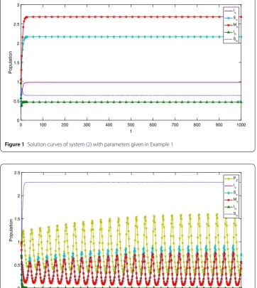
Example1 We takeb1= 0.7978,b2= 0.9020,μh= 0.3485,δh= 0.8706,μv1=μv2= 0.2381, d= 0.8202,β1= 0.9050,β2= 0.6740,α = 0.1464 (all the parameters are stochastically
chosen for illustrative purpose only). Numerical calculations give R01 = 3.1489 > 1 and C1C2–C3= –0.0138 < 0. It follows from Corollary3.1that the disease equilibrium of
sys-tem (2) is locally asymptotically stable, that is, the vector-borne disease will persist in the absence of predators (see Fig.1).
Example2 We take a2= 0.6497,e2= 0.1356,γ2 = 0.7855,h2 = 0.6425 and keep other
Figure 1Solution curves of system (2) with parameters given in Example1
Figure 2Solution curves of system (1) with parameters given in Example2
R02= 0.5331 < 1. It follows from Theorem3.2that the vector-borne disease will tend to
die out (see Fig.2). By calculations,C1C2–C3= –0.0138 < 0, then by Theorem3.4there
exists a stable limit cycle in the (Mv,Sv,P2) space for system (1) (see Fig.3).
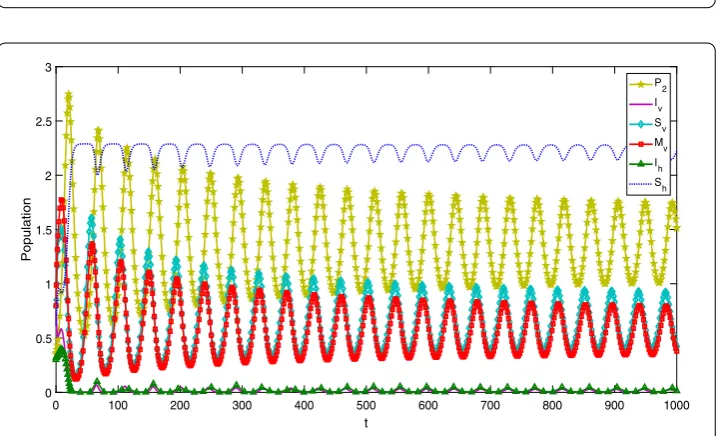
Example3 Keep all the parameters fixed in Example2except forh2= 0.3841. By
calcula-tion the values ofR1andC1C2–C3remain the same as in Example2andR02= 1.0396 > 1,
then by Theorem3.2the vector-borne disease persists, but the equilibrium levels of the infected hosts and vectors have been greatly lessened when the predatorP2is added (see
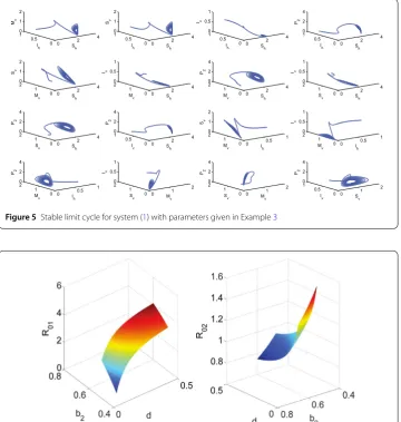
Fig.4). Moreover, Fig.5illustrates that there exists a stable limit cycle for system (1) if
R1> 1,R02< 1, andC1C2–C3< 0.
Example4 Takeμv1= 0.1 and keep all the parameters unchanged in Example1except
Figure 3Stable limit cycle in the (Mv,Sv,P2) space for system (1) with parameters given in Example2
Figure 4Solution curves of system (1) with parameters given in Example3
But ifb2anddare large, then we haveR01> 1. This suggests that in the absence of the
predator, the birth rateb2 of the immature vectors and the conversion rated from the
immature vectors to the mature vectors will cause the spread of the vector-borne disease (see the left-hand side of Fig.6). Takeμv1= 0.1 and keep all the parameters unchanged
in Example2except for parametersb2andd, then from the right-hand side of Fig.6it
is clear that when predators are present, an increase in the vector birth rateb2and the
conversion ratedfrom the immature vectors to the mature vectors will reduce the value of the reproduction numberR02, and therefore lessen the prevalence of disease, because
an increase in the vector birth rate and the conversion rate leads to an increase in the predator population.
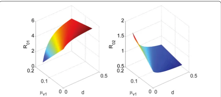
Example5 Takeb2= 0.7343 and keep all the parameters unchanged in Example4except
Figure 5Stable limit cycle for system (1) with parameters given in Example3
Figure 6Surface plot of the basic reproduction numbersR01andR02as functions ofb2anddfor the
parameters given in Example4
But ifdis large anduv1is small, then we haveR01> 1. This suggests that the conversion
ratedfrom the immature vectors to the mature vectors will cause the spread of the vector-borne disease in the absence of predators, while the natural death rateuv1of the immature
vector can reduce the vector disease spread (see the left-hand side of Fig.7). When the predators are introduced, we find from the right-hand side of Fig.7that an increase in the conversion ratedfrom the immature vectors to the mature vectors leads to a decline in the value of the reproduction numberR02, while an increase in the natural death rate
of the immature vectors leads to an increase in the value of the reproduction number
R02, because an increase in the immature vector mortality rateμv1indirectly leads to an
increase in the predator densities.
Remark2 From Figs.2–3and Figs.4–5, it is clear that periodic solutions exist when a predator speciesP2 is introduced in the system, suggesting the occurrence of a
Figure 7Surface plot of the basic reproduction numbersR01andR02as functions ofμv1anddfor the
parameters given in Example5
and mature ones, and the predators oscillate, leading to the persistence of the vector-transmitted disease when the predator speciesP2is added. By enhancing predators’ attack
rateh2, the level of infected hostsIhand vectorsIvwill decline, and whenh2= 0.6425, from
Figs.2–3we can see that predation brings about the extinction of the disease, despite the oscillations between the predators and the vectors. That is to say, introducing predators to vectors is advantageous to vector-borne disease control, and the larger the capturing rateh2is, the better control of disease will be.
Remark3 From the left-hand sides of Figs.6and7, we find that the stage structure has dif-ferent effects on disease transmission dynamics with and without predators. When preda-tors are introduced, small values of the birth rateb2and the conversion rated, and large
value of the natural death rateμv1will lead to the increase in the value of the basic
re-production numberR02, and therefore increase the risk of disease spread. In the absence
of predators, we find that the reproduction numberR01increases with the increase in the
birth rateb2and the conversion ratedof the immature vectors, and with the decrease in
the natural death rateμv1of the immature vectors. Therefore, for vector–host disease
pre-vention and control in the absence of the predator, it is necessary to take some strategies to reduce the birth rateb2and the conversion rated, and enlarge the natural death rate
μv1at vectors’ larva stage, such as use of physical strategies, use of pesticides, biological
control, and so on.
From Sect.3, we find that the predatorP2brings about complicated dynamics of system
(1), and we also find that introducing the predator has certain benefits to disease control. It is clear from Figs.2–5that the larger the value of capturing rateh2is, the lower equilibrium
levels of infected hosts and vectors will be.
5 Conclusions and discussions
among hosts by the mature vectors). The interactions between the predator and the vec-tor are modeled by Holling type II functional response. Corollary3.1reveals that in the absence of the predator, the reproduction numberR01of system (2) provides the threshold
which decides the persistence and extinction of vector-borne diseases. IfR01< 1, the
dis-eases will tend to die out, while ifR01> 1 then the diseases will persist (see Fig.1). When the
predators are added, we find from Theorem3.2that the diseases still persist ifR02> 1, but
the equilibrium levels of the infected hosts and vectors have been lessened (see Fig.2). If
R02< 1, then by Theorem3.2the diseases can be eradicated (see Fig.3). Therefore,
preda-tors have positive effects on disease control. Moreover, by Theorem3.2predation causes the phenomenon of limit cycle arising from a Hopf bifurcation (see Fig.2–5). IfR02< 1 and C1C2–C3> 0, then there exists a stable limit cycle in the (Mv,Sv,P) space for system (1).
Though periodic oscillation occurs between the vectors and the predators, the diseases can be eradicated by the effect of predators on vectors (see Fig.2–3). However, ifR02> 1
andC1C2–C3> 0, then there exists a stable limit cycle for system (1), and the diseases
cannot be eradicated (see Fig.4–5). Finally, the effect of stage structure on disease spread with and without predators has been illustrated (see Fig.6–7). From the left-hand sides of Figs.6and7, it is clear that in the absence of predators, the reproduction numberR01
increases with the increase in the birth rateb2and the conversion ratedof the immature
vectors, whileR01increases with the decrease in the natural death rateμv1of the immature
vectors. Therefore, it is necessary to take some strategies to reduce the birth rateb2and
the conversion ratedand enlarge the natural death rateμv1at vectors’ larva stage through
the use of physical strategies, use of pesticides, biological control, and so on. From the right-hand sides of Figs.6and7, we find that after introducing the predators, the effect ofb2,d, andμv1on disease transmission is inverse compared with the effect ofb2,d, and
μv1on disease transmission in the absence of predators. Therefore, to exert the best effect
of predators on disease control, we should increase the values of the birth rateb2and the
conversion ratedto certain degree, and decrease the value of the natural death rateμv1
of vectors at the immature stage.
Acknowledgements
The authors would like to thank the editor and two anonymous reviewers for their valuable suggestions and comments.
Funding
The work is supported by the National Natural Science Foundation of China (grant no. 71701082 and 71271103), the Six Talents Peak Foundation of Jiangsu Province, and the Innovative Foundation for Doctoral Candidate of Jiangsu Province, China (grant no. CXZZ13_0687).
Competing interests
The authors declare that they have no competing interests.
Authors’ contributions
All authors contributed equally to the writing of this paper. All authors read and approved the final manuscript.
Author details
1Department of Mathematics, Shaoxing University, Shaoxing, P.R. China.2School of Mathematics and Statistics, Central
South University, Changsha, P.R. China. 3Faculty of Science, Jiangsu University, Zhenjiang, P.R. China.4College of Civil
Engineering, Shaoxing University, Shaoxing, P.R. China.5School of Finance and Economics, Jiangsu University, Zhenjiang,
P.R. China.
Publisher’s Note
Springer Nature remains neutral with regard to jurisdictional claims in published maps and institutional affiliations.
References
1. Jones, K.E., Patel, N.G., Levy, M.A., Storeygard, A., Balk, D., Gittleman, J.L., Daszak, P.: Global trends in emerging infectious diseases. Nature451, 990–993 (2008)
2. Daszak, P., Cunningham, A., Hyatt, A.D.: Anthropogenic environmental change and the infectious diseases in wildlife. Acta Trop.78, 103–116 (2001)
3. Yang, C.X., Nie, L.F.: Modelling the use of impulsive vaccination to control Rift Valley Fever virus transmission. J. Differ. Equ.2016, 134 (2016)
4. Nie, L.F., Xue, Y.N.: The roles of maturation delay and vaccination on the spread of Dengue virus and optimal control. J. Differ. Equ.2017, 278 (2017)
5. Hemingway, J., Ranson, H.: Insecticide resistance in insect vectors of human disease. Annu. Rev. Entomol.45, 371–391 (2000)
6. Castro, M.C., De Yamagata, Y., Mtasiwa, D., Tanner, M., Utzinger, J., Keiser, J., Singer, B.H.: Integrated urban malaria control: a case study in Dares Salaam, Tanzania. Am. J. Trop. Med. Hyg.71, 103–117 (2004)
7. Benedict, M.Q., Robinson, A.S.: The first releases of transgenic mosquitoes: an argument for the sterile insect technique. Trends Parasitol.19, 349–355 (2003)
8. Kaaya, G.P., Hassan, S.: Entomogenous fungi as promising biopesticides for tick control. Exp. Appl. Acarol.24, 913–926 (2000)
9. Scholte, E.J., Ng’Habi, K., Kihonda, J., Takken, W., Paaijmans, K., Abdulla, S., Killeen, G.F., Knols, B.G.J.: An entomopathogenic fungus for control of adult African malaria mosquitoes. Science308, 1641–1642 (2005) 10. Legner, E.: Biological control of Diptera of medical and veterinary importance. J. Vector Ecol.20, 59–120 (1995) 11. Stauffer, J.R. Jr., Arnegard, M., Cetron, M.: Controlling vectors and hosts of parasitic diseases using fishes. Bioscience
47, 41–49 (1997)
12. Samish, M., Rehacek, J.: Pathogens and predators of ticks and their potential in biological control. Annu. Rev. Entomol. 44, 159–182 (1999)
13. Ostfeld, R.S., Price, A., Hornbostel, V.L., Benjamin, M.A., Keesing, F.: Controlling ticks and tick-borne zoonoses with biological and chemical agents. Bioscience56, 383–394 (2006)
14. Walker, K., Lynch, M.: Contributions of Anopheles larval control to malaria suppression in tropical Africa: review of achievements and potential. Med. Vet. Entomol.21, 2–21 (2007)
15. Ghosh, S.K., Tiwari, S.N., Sathyanarayan, T.S., Sampath, T.R., Sharma, V.P., Nanda, N., Joshi, H., Adak, T., Subbarao, S.K.: Larvivorous fish in wells target the malaria vector sibling species of the Anopheles culicifacies complex in villages in Karnataka, India. Trans. R. Soc. Trop. Med. Hyg.99, 101–105 (2005)
16. Ghosh, S.K., Dash, A.P.: Larvivorous fish against malaria vectors: a new outlook. Trans. R. Soc. Trop. Med. Hyg.101, 1063–1064 (2007)
17. Kay, B., Nam, V.S.: New strategy against Aedes aegypti in Vietnam. Lancet365, 613–617 (2005)
18. Kittayapong, P., Yoksan, S., Chansang, U., Chansang, C., Bhumiratana, A.: Suppression of dengue transmission by application of integrated vector control strategies at sero-positive GIS-based foci. Am. J. Trop. Med. Hyg.78, 70–76 (2008)
19. Zhang, L.Q., Liu, J., Wu, H.: The screening of a virulent strain of Beauveria bassiana to Monochamus alternatus. J. Nanjing For. Univ.24, 33–37 (2000)
20. Lai, Y.X., Liu, J.D., Xu, Q.Y., Wang, Y.H., Zhou, C.M.: Trials on the parasitism of Beauveria bassiana or Verticillium lecanii on larvae of Monochamus alternatus Hope. J. Jiangsu. For. Sci. Technol.30, 7–9 (2003)
21. Jeger, M.J., Holt, J., Van Den Bosch, F., Madden, L.V.: Epidemiology of insect-transmitted plant viruses: modelling disease dynamics and control interventions. Physiol. Entomol.29, 291–304 (2004)
22. Otim, M., Legg, D., Kyamanywa, S., Polaszek, A., Gerling, D.: Population dynamics of Bemisia tabaci (Homoptera: Aleyrodidae) parasitoids on cassava mosaic disease-resistant and susceptible varieties. Biocontrol Sci. Technol.16, 205–214 (2006)
23. Luck, R.F., Shepard, B.M., Kenmore, P.E.: Experimental methods for evaluating arthropod natural enemies. Annu. Rev. Entomol.33, 367–389 (1988)
24. Zehnder, G., Gurr, G.M., Kühne, S., Wade, M.R., Wratten, S.D., Wyss, E.: Arthropod pest management in organic crops. Annu. Rev. Entomol.52, 57–80 (2007)
25. Tian, B.D., Yang, L., Zhong, S.M.: Global stability of a predator–prey model with Allee effect. Int. J. Biomath.8, 37–51 (2015)
26. Zha, L.J., Cui, J.A., Zhou, X.Y.: Ratio-dependent predator-prey model with stage structure and time delay. Int. J. Biomath.5, 15–37 (2012)
27. Zhou, F.Y.: Existence and global attractivity of a positive periodic solution for a non-autonomous predator-prey model under viral infection. Int. J. Biomath.2, 419–442 (2009)
28. Schraiber, J.G., Kaczmarczyk, A.N., Kwok, R., et al.: Constraints on the use of lifespan-shortening Wolbachia to control dengue fever. J. Theor. Biol.297, 26–32 (2012)
29. Hughes, H., Britton, N.F.: Modelling the use of Wolbachia to control dengue fever transmission. Bull. Math. Biol.75, 796–818 (2013)
30. Moore, S.M., Borer, E.T., Hosseini, P.R.: Predators indirectly control vector-borne disease: linking predator-prey and host-pathogen models. J. R. Soc. Interface7, 161–176 (2009)
31. Zhou, F.Y., Yao, H.Y.: Dynamics and biocontrol: the indirect effects of a predator population on a host-vector disease model. Abstr. Appl. Anal.2014, 252718 (2014)
32. Okamoto, K.W., Amarasekare, P.: The biological control of disease vectors. J. Theor. Biol.309, 47–57 (2012) 33. Xiao, Y.N., Chen, L.S.: An SIS epidemic model with stage structure and a delay. Acta Math. Appl. Sin.18, 607–618
(2002)
34. Cai, L., Li, X., Ghosh, M.: Global stability of a stage-structured epidemic model with a nonlinear incidence. Appl. Math. Comput.214, 73–82 (2009)
35. Hyman, J.M., Li, J., Stanley, E.A.: The differential infectivity and staged progression models for the transmission of HIV. Math. Biosci.155, 77–109 (1999)
37. Martcheva, M., Castillo-Chavez, C.: Diseases with chronic stage in a population with varying size. Math. Biosci.182, 1–25 (2003)
38. Tian, B.D., Jin, Y.G., Zhong, S.M., Chen, N.: Global stability of an epidemic model with stage structure and nonlinear incidence rates in a heterogeneous host population. J. Differ. Equ.2015, 260 (2015)
39. World health organization: Frequently Asked Questions Scrub Typhus (2008)
40. Zhao, B.G., Futai, K., Jack, R., Sutherland, J.R., Takeuchi, Y.: Pine Wilt Disease. Springer, New York (2008)
41. Diekmann, O., Heesterbeek, J.A.P., Metz, J.A.J.: On the definition and the computation of the basic reproduction ratio R0in models for infectious diseases in heterogeneous populations. J. Math. Biol.28, 365–382 (1990)
42. Driessche, V.P., Watmough, J.: Reproduction numbers and sub-threshold endemic equilibria for compartmental models of disease transmission. Math. Biosci.180, 29–48 (2002)