R E S E A R C H
Open Access
An expanded mixed covolume element
method for integro-differential equation of
Sobolev type on triangular grids
Zhichao Fang
*, Hong Li, Yang Liu and Siriguleng He
*Correspondence:
[email protected] School of Mathematical Sciences, Inner Mongolia University, Hohhot, 010021, China
Abstract
The expanded mixed covolume Element (EMCVE) method is studied for the two-dimensional integro-differential equation of Sobolev type. We use a piecewise constant function space and the lowest order Raviart-Thomas (RT0) space as the trial
function spaces of the scalar unknownuand its gradientσand fluxλ, respectively. The semi-discrete and backward Euler fully-discrete EMCVE schemes are constructed, and the optimal a priori error estimates are derived. Moreover, numerical results are given to verify the theoretical analysis.
MSC: 65M08; 65M60
Keywords: integro-differential equation of Sobolev type; expanded mixed covolume element method; optimal a priori error estimate
1 Introduction
We consider the linear integro-differential equation of Sobolev type
c(x)∂u
∂t –div
a(x)∇u+b(x)∇∂u
∂t + t
k(x,t,τ)∇u(x,τ) dτ
=f(x,t), ()
for (x,t)∈×J, with boundary and initial conditions
⎧ ⎨ ⎩
u(x,t) = , (x,t)∈∂× ¯J,
u(x, ) =u(x), x∈,
()
where is a convex and bounded polygonal domain inR with boundary denoted by ∂,J= (,T] with <T<∞, the initial functionu(x), the source functionf(x,t), and
coefficientsk(x,t,τ),a(x),b(x) andc(x) are given bounded and smooth functions, and there exist some constantsa,a,b,b,candcsuch that
<a≤a(x)≤a<∞, <b≤b(x)≤b<∞, <c≤c(x)≤c<∞.
Partial integro-differential equations are often used to describe various physical pro-cesses such as heat conduction behavior in memory material, nuclear reactor dynamics, compression of viscoelastic media and the propagation of sound in viscous media.
ious numerical studies have been reported based on the finite element methods [–], finite volume element methods [, ], mixed finite element methods [–], discontinu-ous mixed covolume methods [] etc. Numerical solutions for the integro-differential equation of Sobolev type have been given by Cui [] who constructed a finite element scheme and obtained optimal error estimate by introducing Sobolev-Volterra projection; Che et al. [] who consideredH-Galerkin expanded mixed finite element method; and
Guezane-Lakoud et al. [] who developed Rothe’s method for one-dimensional problem with integral conditions.
Mixed covolume element (MCVE) method was first introduced by Russell [] to solve the mixed formulation of linear elliptic problems. Subsequently, Chou et al. [, ] consid-ered the MCVE method for the elliptic boundary value problems by using theRTspace
on the triangular grids and rectangular grids, respectively. This method not only can cal-culate several different physical quantities (such as pressure and Darcy velocity in []) but also maintains the mass local conservation law, and this is very important in fluid numeri-cal computations. The satisfactory numerinumeri-cal simulation results on different test problems were obtained in [–]. The MCVE methods have been used to solve quasi-linear sec-ond order elliptic equations [], parabolic equations [, ], and so on.
This article proposes an EMCVE scheme to solve the D linear integro-differential equation of Sobolev type. We introduce the variables σ(x,t) = –∇u(x,t) and λ(x,t) = –(a(x)∇u(x,t) +b(x)∇ut+
t
k(x,t,τ)∇u(x,τ) dτ) and write problem () as the system of
first order PDEs
⎧ ⎪ ⎪ ⎨ ⎪ ⎪ ⎩
(a) σ(x,t) = –∇u(x,t),
(b) λ(x,t) =a(x)σ(x,t) +b(x)∂∂tσ(x,t) +tk(x,t,τ)σ(x,τ) dτ, (c) c(x)∂u∂t(x,t) +divλ(x,t) =f(x,t).
()
The EMCVE scheme is obtained by integrating these equations on local covolume di-rectly and using the Green’s formula when proper. And then, the local conservation law with the discrete solution holds. This method skillfully combines finite volume element methods [, ] with expanded mixed finite element methods [, ], can use the ad-vantage of finite volume element methods to calculate more different physical quantities simultaneously. Rui and Lu [] applied the EMCVE method to solve the elliptic problem on rectangular grids in the rectangular area. In this article, we propose a semi-discrete and backward Euler fully-discrete EMCVE scheme based on triangular grids and obtain the optimal order error estimates by introducing a Volterra-type generalized EMCVE projec-tion. Moreover, we give numerical results for a model equation to verify the feasibility and effectiveness of the scheme.
The expanded mixed weak formulation of () is to solve (u,σ,λ)∈L()×H(div,)×
H(div,) satisfying
⎧ ⎪ ⎪ ⎪ ⎪ ⎪ ⎨ ⎪ ⎪ ⎪ ⎪ ⎪ ⎩
(σ, w) – (divw,u) = , ∀w∈H(div,), (λ, z) = (aσ, z) + (bσt, z) + (
t
kσdτ, z), ∀z∈H(div,),
(cut,v) + (divλ,v) = (f,v), ∀v∈L(),
u(x, ) =u(x), σ(x, ) = –∇u(x), ∀x∈,
()
We also use the general notations and definitions of the Sobolev spaces as in []. Let (·,·) be the inner product inL() and (L()), that is, (ψ,φ) =
ψ φdx(ifψ,φ∈L
()) and
(z, w) =z·wdx(if z, w∈(L())), and either · L()or · (L())is denoted as · .
We also use the normzH(div,)= (z+divz)
of the space H(div,). Throughout
this paper, the constantC> does not depend on the spatial and time mesh parameters
handt.
2 Expanded mixed covolume element formulation
In order to describe the EMCVE scheme for system (), we construct the partitionTh of
the domain. As in [], letTh={KB}be a quasi-uniform triangulation partition, where
KBis the triangle with barycenter pointB, andh=max{hKB},hKBstands for the diameter of triangleKB. We define the nodes to be the midpoints on the edges of every triangular
el-ement, whereP,P, . . . ,PNτstand for interior nodes, andPNτ+, . . . ,PNstand for boundary nodes.
We use theRTspace as the trial function space Hhfor variablesσ andλ, where
Hh=
zh∈H(div,) : zh|K= (a+bx,c+bx),∀K∈Th
, ()
and useLhas a trial space for variableu, where
Lh=
vh∈L() :vh|Kis constant,∀K∈Th
. ()
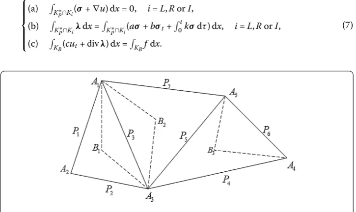
Now the dual partitionTh∗is constructed by a union of interior quadrilaterals and border triangle. Referring now to Figure , and the quadrilateralABABis the dual elementKP∗
with interior nodeP, which contains two elementsKL(the triangle ABA) andKR(the
triangle AAB); the triangle AABis the dual elementKP∗with boundary nodeP,
which contains one elementKI(the triangle ABA).
Integrate () on these primal and dual elements to obtain
⎧ ⎪ ⎪ ⎪ ⎨ ⎪ ⎪ ⎪ ⎩
(a) K∗
P∩Ki(σ+∇u) dx= , i=L,RorI, (b) K∗
P∩Kiλdx=
KP∗∩Ki(aσ+bσt+
t
kσdτ) dx, i=L,RorI,
(c) K
B(cut+divλ) dx=
KBfdx.
()
Similar to [, ], we define a transfer operatorγh: Hh→(L())by
γhzh= Nτ
j=
zh|KL(Pj)χKj∗∩KL+ zh|KR(Pj)χKj∗∩KR
+
N
j=Nτ+
zh|KI(Pj)χKj∗, ()
whereχKmeans the characteristic function of a setK. Then we choose the range ofγhas
the test function space Yh. By using the transfer operatorγh, we can rewrite equations (a)
and (b) in () as
(σ+∇u,γhwh) = , ∀wh= Hh, ()
(λ,γhzh) =
aσ+bσt+
t
kσdτ,γhzh
, ∀zh= Hh. ()
Applying Green’s integral formula, we have
(∇u,γhwh) = N
j=Nτ+
wh|KI(Pj)
∂KPj∗\∂
vhndλ
+
Nτ
j=
wh|KL(Pj)
∂KPj∗∩KL
vhndλ+ wh|KR(Pj)
∂KPj∗∩KR
vhndλ
≡b(γhwh,u),
for∀wh∈Hh, where n stands for the unit out-normal direction.
By calculation, it is easy to get the equality b(γhwh,vh) = –(divwh,vh), ∀wh ∈Hh, ∀vh∈Lh. Then we can obtain the semi-discrete EMCVE scheme to find (uh,σh,λh)∈
Lh×Hh×Hhsuch that
⎧ ⎪ ⎪ ⎨ ⎪ ⎪ ⎩
(σh,γhwh) – (divwh,uh) = , ∀wh∈Hh,
(λh,γhzh) = (aσh,γhzh) + (bσht,γhzh) + (
t
kσhdτ,γhzh), ∀zh∈Hh,
(cuht,vh) + (divλh,vh) = (f,vh), ∀vh∈Lh,
()
and the initial valuesuh() andσh() will be defined in Theorems . and ..
3 Some lemmas
For∀zh= (zh,zh)∈Hh, the discrete norms are defined as follows:
|zh|,h=
K∈Th
∇z
h
,K+∇z
h
,K
, zh,h=zh+|zh|,h.
Lemma .([]) The operatorγhis bounded
and satisfies
(I–γh)zh≤Chzh,h, ∀zh∈Hh,
zh, (I–γh)wh≤Chzh,hwh, ∀zh, wh∈Hh,
z, (I–γh)wh≤Chzwh, ∀z∈
H(),∀wh∈Hh.
Lemma .([]) The following symmetry relation
(γhzh, wh) = (zh,γhwh), ∀zh, wh∈Hh,
holds,and there is a constantμ> independent of h such that
(γhzh, zh)≥μzh, ∀zh∈Hh.
For∀x∈KB, we definea¯(x) =a(B),b¯(x) =b(B),k¯(x,t,τ) =k(B,t,τ).
Lemma .([]) The following symmetry relation
(a¯γhzh, wh) = (a¯zh,γhwh), ∀zh, wh∈Hh,
(b¯γhzh, wh) = (b¯zh,γhwh), ∀zh, wh∈Hh,
holds,and there are constantsμ> ,μ> independent of h such that
(azh,γhwh) – (a¯zh,γhwh)≤Chzhwh, ∀zh, wh∈Hh,
(bzh,γhwh) – (b¯zh,γhwh)≤Chzhwh, ∀zh, wh∈Hh,
(a¯zh,γhzh)≥μzh, (azh,γhzh)≥μzh, ∀zh∈Hh,
(b¯zh,γhzh)≥μzh, (bzh,γhzh)≥μzh, ∀zh∈Hh.
Lemma .([]) The following estimates hold:
azh, (I–γh)wh≤Chzh,hwh, ∀zh, wh∈Hh,
az, (I–γh)wh≤Chzwh, ∀z∈
H(),∀wh∈Hh,
bzh, (I–γh)wh≤Chzh,hwh, ∀zh, wh∈Hh,
bz, (I–γh)wh≤Chzwh, ∀z∈
H(),∀wh∈Hh.
The Raviart-Thomas projectionh: H(div,)→Hhis defined in [] such that
div(z –hz),vh
= , ∀z∈H(div,),∀vh∈Lh,
and theLprojectionR
h:L()→Lhis defined by
Then the properties ofhandRhare known from [–]
Lemma .([]) The following estimate holds:
z–γhhz ≤Chz, ∀z∈
H().
Lemma . The following symmetry relation
t
By applying the numerical quadrature formula, we get
To prove (), using (), we have
Noting thatk(x,t,τ) is Lipschitz continuous with variablex, we get the desired
conclu-sion.
Proof To prove (), we obtain
t
By using Lemmas . and ., we complete the proof of (). Next we prove (). Using (), we have
Theorem . Suppose(u˜h,σ˜h,λ˜h)satisfies(a)-(c),then there is a constant C>
inde-pendent of h and t such that
λ–λ˜h ≤Chλ, ()
div(λ–λ˜h)≤Chdivλ, ()
σ–σ˜h ≤Ch
σ+λ+ t
σdτ
, ()
u–u˜h ≤Ch
σ+λ+u+ t
σdτ
. ()
Proof Noting thatλ˜h=hλ, we have estimates () and ().
Splittingσ–σ˜h=σ–hσ+hσ–σ˜hin (c) yields
a(hσ–σ˜h),γhzh
= (λ–λ˜h,γhzh) +
λ, (I–γh)zh
–
t
k(σ–σ˜h) dτ,γhzh
–
t
kσdτ, (I–γh)zh
–aσ, (I–γh)zh
–a(σ–hσ),γhzh
, ∀zh∈Hh. ()
Choose zh=hσ–σ˜hin () and use the Cauchy-Schwarz inequality to get
μhσ–σ˜h≤C
λ–λ˜h+σ–hσ
+Chλ+σ
+C t
σ–hσ+hσ+hσ–σ˜h
dτ
+μ
hσ–σ˜h
. ()
Using () and (), applying Gronwall’s inequality, we obtain estimate ().
Noting thatdiv(Hh) =Lh, we have (divwh,u–Rhu) = ,∀wh∈Hh, and rewrite (b) as
(σ–σ˜h,γhwh) – (divwh,Rhu–u˜h) = –
σ, (I–γh)wh
, ∀wh∈Hh. ()
Next we introduce an auxiliary elliptic problem. Givenϕ∈L(), letψ satisfy the
fol-lowing elliptic problem:
⎧ ⎨ ⎩
–ψ=ϕ, x∈,
ψ= , x∈∂. ()
And we have the following elliptic regularity result:
ψ≤Cϕ. ()
Using the projectionhandRh, and ()-(), we have
(Rhu–u˜h,g) = (Rhu–u˜h, –ψ) = –
divh(∇ψ)
,Rhu–u˜h
= –σ, (I–γh)
h(∇ψ)
–σ–σ˜h,γhh(∇ψ)
= –σ, (I–γh)
Apply the triangle inequality with () and () to obtain ().
Differentiating (a)-(c) with respect to time variablet, we can also obtain the follow-ing projection estimates.
Theorem . Suppose(u˜h,σ˜h,λ˜h)satisfies(a)-(c),then there is a constant C>
in-dependent of h and t such that
4 The error estimates of semi-discrete expanded mixed covolume element formulation
In this section, we first discuss the existence and uniqueness of solution for the semi-discrete EMCVE scheme ().
Theorem . Set uh() =u˜h(),σh() =σ˜h(),then there is a unique solution for system
Proof Let{χj}N
It is easy to see thatAandCare symmetric positive definite matrixes, andA andA
are invertible matrixes. We rewrite equation (c) in () as
⎧
Using quadratic form theory, we can know that (A+G–) is an invertible matrix, and
problem () has a unique solution by the theory of differential equations. Thus, systems
() and () have a unique solution.
Now we write the errors as
σ–σh=σ–σ˜h+σ˜h–σh=ξ˜+ξ,
λ–λh=λ–λ˜h+λ˜h–λh=ζ˜+ζ,
where (u˜h,σ˜h,λ˜h) is the Volterra-type generalized EMCVE projection of (u,σ,λ). Using
() and (), we have the error equations
(ξ,γhwh) – (divwh,φ) = , ∀wh∈Hh, (a)
Proof Differentiating (a) with respect to variablet, we have
Integrating the above inequality from tot, we get
Integrating () from totyields
cφ–cφ()+μ
Using Gronwall’s inequality yields
Substituting () and () into () yields
cφt+μξt≤C
˜φt+˜ξt+hσt
+C t
˜φt+˜ξt+hσt
dt. ()
To estimateλ–λhandλ–λhH(div,), we choose zh=ζ in (b) to see that
(ζ,γhζ) = (aξ,γhζ) + (bξt,γhζ) +
bσt, (I–γh)ζ
+ (bξ˜t,γhζ) +
t
kξdτ,γhζ
.
Using Lemmas . and ., we get
μζ≤C
ξt+ξ+˜ξt+hσt+C t
ξdτ+μ ζ
. ()
Substituting (), () and () into (), we have that
ζ≤C ˜φt+˜ξt+hσt
+C t
˜φt+˜ξt+hσt
dt. ()
Choosingvh=divζ in (c) yields
(divζ,divζ) = –(cφt,divζ) – (cφ˜t,divζ).
And we have
divζ≤C ˜φt+φt.
Using () and (), we have
divζ≤C˜ξt+ ˜φt+hσt
+C t
˜ξt+ ˜φt+hσt
dt. ()
Thus, combine (), (), () and (), apply the triangle inequality to complete the
proof.
5 The fully-discrete expanded mixed covolume element formulation
Lettbe the time step length, andtn=nt(n= , , , . . . ,M) for some positive integerM.
Defineϕn=ϕ(tn) and∂tϕn=ϕ
n–ϕn–
t for a functionϕ. To approximate the integral term,
we select the left rectangle quadrature formula
tn
ϕ(s) ds≈t
n–
j= ϕ(tj),
and the quadrature errorεn(ϕ) =tn
ϕ(s) ds–t n–
j=ϕ(tj) satisfies
εn(ϕ)≤Ct
tn
Now, we define the backward Euler fully-discrete scheme: find (unh,σnh,λnh)∈Lh×Hh×
(b). The calculation proceeds by solving (c), (d) and (e) equations for{σn h,λnh,unh}
with using already calculated{σn–
h ,unh–}. It is easy to get that there is a unique solution
for the fully-discrete scheme (a)-(e). We now rewrite the errors as
σ(tn) –σnh=σ(tn) –σ˜h(tn) +σ˜h(tn) –σnh=ξ˜n+ξn,
λ(tn) –λnh=λ(tn) –λ˜h(tn) +λ˜h(tn) –λnh=ζ˜n+ζn,
u(tn) –unh=u(tn) –u˜h(tn) +u˜h(tn) –unh=φ˜n+φn,
where (u˜h,σ˜h,λ˜h) is the Volterra-type generalized EMCVE projection of (u,σ,λ).
Using (a)-(c), we obtain the following error equations:
Theorem . Let(unh,σnh,λnh)be the solution of scheme(a)-(e),and suppose that the
so-Proof Using (a)-(c), we rewrite (b) as
Note that (a¯ξm,γ
hξm)≥μξm, choosetin () to satisfyCt<μ, and use
Gron-wall’s inequality to get
ξm≤Cξ+Ct
Now, by Lemma ., it follows from () that
c∂tφn
Substituting () into (), we have that
c∂tφn
Substituting () and () into (), we have
Substituting () into (), we get
, and use Gronwall’s inequality to get
φm≤Cφ+ξ+Ct
Now, we note that
βn≤Ct
Using (a)-(c), we have
˜σh≤C
Further, using (a) and (b), we get
ξ≤
Chσ()+λ(), ()
φ≤φ˜≤Chu()+σ()+λ(). ()
Finally, apply the triangle inequality to obtain the error estimates.
6 Numerical example
For confirming the above theoretical analysis, we give a numerical example and consider the spatial and temporal domain= (, )×(, ),J= (, ], the coefficientsa(x) = + x
+x,b(x) = +x+ x,c(x) = ,k(x,t,τ) = ( +x+x+t)τ, and the initial function
u(x, ) =x(x– )x(x– ).
The exact solution is
u(x,t) =e–tx(x– )x(x– ),
backward Euler fully-discrete scheme are given in Table by usingRTspace with different
mesh sizesh=√t=
. Based on the error results and convergence rates,
we can verify the theoretical analysis.
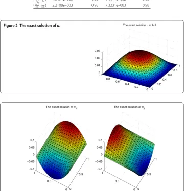
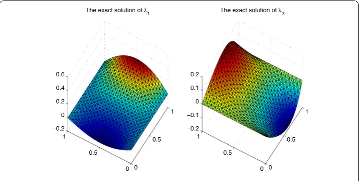
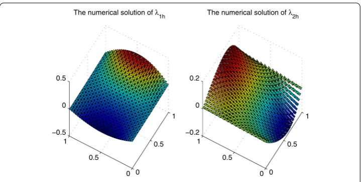
The graphs of exact solutions foru,σ andλatt= are drawn on Figures , and , respectively. The graphs of the corresponding discrete solutions forunh,σnh andλnh with the meshh=
√
andt=
are drawn on Figures , and , respectively. The numerical
Table 1 Error estimates and convergence rates
h,t u – uhL∞(L2()) Rate σ–σhL∞((L2())2) Rate
( √
2 8 ,
1
8) 3.8464e–003 1.6043e–002
(√2 16,
1
16) 2.0591e–003 0.90 8.6877e–003 0.88
(√322,321) 1.0637e–003 0.95 4.5181e–003 0.94 (
√ 2 64,
1
64) 5.4043e–004 0.98 2.3037e–003 0.97
h,t λ–λhL∞((L2())2) Rate λ–λL∞(H(div,)) Rate
(√82,1
8) 1.5432e–002 5.1929e–002
(√162,161) 8.3902e–003 0.88 2.7873e–002 0.90 (
√ 2 32,
1
32) 4.3491e–003 0.95 1.4411e–002 0.95
(√2 64,
1
64) 2.2108e–003 0.98 7.3231e–003 0.98
Figure 2 The exact solution ofu.
Figure 3 The exact solution ofσ= (σ1,σ2).
7 Conclusions
We present the EMCVE method for the D linear integro-differential equation of Sobolev type. We introduce the transfer operatorγh and construct the semi-discrete, backward
Euler fully-discrete EMCVE schemes. We obtain the optimal order error estimates for the scalar unknownu(inL()-norm), gradientσ(in (L())-norm) and fluxλ(in (L())
Figure 4 The exact solution ofλ= (λ1,λ2).
Figure 5 The numerical solution ofuh.
Figure 7 The numerical solution ofλh= (λ1h,λ2h).
Competing interests
The authors declare that they have no competing interests.
Authors’ contributions
All authors contributed equally to the writing of this paper. All authors read and approved the final manuscript.
Acknowledgements
This work was supported by the National Natural Science Fund of China (11661058, 11361035, 11501311), the Natural Science Fund of Inner Mongolia Autonomous Region (2016BS0105, 2016MS0102, 2017MS0107), the Scientific Research Projection of Higher Schools of Inner Mongolia (NJZY14013), the Program of Higher-Level Talents of Inner Mongolia University (30105-135127).
Publisher’s Note
Springer Nature remains neutral with regard to jurisdictional claims in published maps and institutional affiliations.
Received: 18 December 2016 Accepted: 10 May 2017 References
1. Lin, YP, Thomée, V, Wahlbin, LB: Ritz-Volterra projections to finite-element spaces and applications to integrodifferential and related equations. SIAM J. Numer. Anal.28, 1047-1070 (1991)
2. Zhang, T, Li, CJ: Superconvergence of finite element approximations to parabolic and hyperbolic integro-differential equations. Northeast. Math. J.17, 279-288 (2001)
3. Pani, AK, Sinha, RK: Error estimates for semidiscrete Galerkin approximation to a time dependent parabolic integro-differential equation with nonsmooth data. Calcolo37, 181-205 (2000)
4. Zhang, T, Lin, YP, Tait, RJ: On the finite volume element version of Ritz-Volterra projection and applications to related equations. J. Comput. Math.5, 491-504 (2002)
5. Li, HR, Li, Q: Finite volume element methods for nonlinear parabolic integro-differential problems. J. Korean Soc. Ind. Appl. Math.7, 35-49 (2003)
6. Sinha, RK, Ewing, RE, Lazarov, RD: Mixed finite element approximations of parabolic integro-differential equations with nonsmooth initial data. SIAM J. Numer. Anal.47, 3269-3292 (2009)
7. Liu, Y, Fang, ZC, Li, H, He, S, Gao, W: A new expanded mixed method for parabolic integro-differential equations. Appl. Math. Comput.259, 600-613 (2015)
8. Shi, DY, Wang, HH: AnH1-Galerkin nonconforming mixed finite element method for integrodifferential equation of
parabolic type. J. Math. Res. Exposition29, 871-881 (2009)
9. Liu, Y, Li, H, Wang, JF, Gao, W: A new positive definite expanded mixed finite element method for parabolic integrodifferential equations. J. Appl. Math.2012, Article ID 391372 (2012)
10. Zhu, AL: Discontinuous mixed covolume methods for linear parabolic integrodifferential problems. J. Appl. Math.
2014, Article ID 649468 (2014)
11. Cui, X: Sobolev-Volterra projection and numerical analysis of finite element methods for integrodifferential equations. Acta Math. Appl. Sin.24, 442-455 (2001)
12. Che, HT, Zhou, ZJ, Jiang, ZW, Wang, YJ:H1-Galerkin expanded mixed finite element methods for nonlinear
pseudo-parabolic integro-differential equations. Numer. Methods Partial Differ. Equ.29, 799-817 (2013)
13. Guezane-Lakoud, A, Belakroum, D: Time-discretization schema for an integrodifferential Sobolev type equation with integral conditions. Appl. Math. Comput.218, 4695-4702 (2012)
15. Chou, SH, Kwak, DY, Vassilevski, PS: Mixed covolume methods for the elliptic problems on triangular grids. SIAM J. Numer. Anal.35, 1850-1861 (1998)
16. Chou, SH, Kwak, DY: Mixed covolume methods on rectangular grids for elliptic problems. SIAM J. Numer. Anal.37, 758-771 (2000)
17. Cai, Z, Jones, JE, Mccormick, SF, Russell, TF: Control-volume mixed finite element methods. Comput. Geosci.1, 289-315 (1997)
18. Kwak, DY, Kim, KY: Mixed covolume methods for quasi-linear second-order elliptic problems. SIAM J. Numer. Anal.38, 1057-1072 (2000)
19. Rui, HX: Symmetric mixed covolume methods for parabolic problems. Numer. Methods Partial Differ. Equ.18, 561-583 (2002)
20. Yang, SX, Jiang, ZW: Mixed covolume method for parabolic problems on triangular grids. Appl. Math. Comput.215, 1251-1265 (2009)
21. Yu, CH, Li, YH: Biquadratic finite volume element method based on optimal stress points for second order hyperbolic equations. Numer. Methods Partial Differ. Equ.29, 738-756 (2013)
22. Zhang, ZY: Error estimates of finite volume element method for the pollution in groundwater flow. Numer. Methods Partial Differ. Equ.25, 259-274 (2008)
23. Chen, Z: Expanded mixed element methods for linear second-order elliptic problems (I). RAIRO Modél. Math. Anal. Numér.32, 479-499 (1998)
24. Chen, Z: Expanded mixed element methods for quasilinear second-order elliptic problems (II). RAIRO Modél. Math. Anal. Numér.32, 501-520 (1998)
25. Rui, HX, Lu, TC: An expanded mixed covolume method for elliptic problems. Numer. Methods Partial Differ. Equ.21, 8-23 (2005)
26. Adams, R: Sobolev Spaces. Academic Press, New York (1975)
27. Fang, ZC, Li, H: An expanded mixed covolume method for Sobolev equation with convection term on triangular grids. Numer. Methods Partial Differ. Equ.29, 1257-1277 (2013)
28. Luo, ZD: Mixed Finite Element Methods and Applications. Chinese Science Press, Beijing (2006) 29. Brezzi, F, Fortin, M: Mixed and Hybrid Finite Element Methods. Springer, New York (1991)