R E S E A R C H
Open Access
Chaos control with STM of minor component
analysis learning algorithm
Lin Zuo
1*and Bin Zhou
2Abstract
One of the most important techniques of feature extraction, i.e., the minor component analysis (MCA), has been widely employed in the field of data analysis. In order to meet the demands of real time computing and curtail the computational complexity, one instrument is often applied, namely, the MCA neural networks, whose learning algorithm, under some conditions, however, can produce complex dynamic behaviors, such as periodical
oscillation, bifurcation, and chaos. This article introduces the chaotic dynamics theory to fully and correctly comprehend the numerical instability and chaos of iterative solutions in the MCA. Especially, as an illustration, the Douglas’MCA chaos control is discussed in details, where a stability transformation method (STM) of chaos feedback control is used in the MCA convergence control. As the time series diagrams, Jacobian matrix and Lyapunov exponent of discrete dynamic system indicate, the desired fixed points of iterative map of Douglas’MCA can be captured and the chaotic behavior of the algorithm can be controlled in the original chaotic interval.
Keywords:Douglas’s MCA, chaos control, stability transformation method, Jacobian matrix, Lyapunov exponent
1. Introduction
Minor component is the small eigenvalue of the correla-tion matrix corresponding to the input dataset, and the MCA is an important technique for data analysis. It can extract the key features of data and its neural network can be used to extract minor components without cal-culating the correlation matrix advance, which makes it an ideal method to decrease the computational com-plexity and thus to be broadly applied in real time appli-cations of data analysis and signal processing [1], such as moving target indication [2], curve and surface fitting [3], total least squares (TLS) [4], clutter cancellation [5], frequency estimation [6], digital beamforming [7], etc. Recently, some MCA learning algorithm are proposed to update the net weights, such as Douglas’s algorithm, where abundant chaos phenomena are detected [8].
MCA learning algorithms usually are described by sto-chastic discrete time (SDT) systems, but it is very diffi-cult to investigate the convergence of the SDT models directly [9]. Consequently, deterministic continuous time (DCT) system associated with the SDT model is
analyzed [10]. Furthermore, because of computational round-off limitations and tracking requirements, the condition corresponding to stochastic approximation theorem can not be satisfied in application easily, so that the convergence of original algorithm can be inter-preted by examining a deterministic discrete time (DDT) system. Actually, the convergence issue of MCA algorithm has been explored according to the corre-sponding DDT system [1,11-13].
On the other side, in essence, the iterative algorithm of nonlinear system xk+1 =f(xk) is a discrete dynamic
system. From the chaotic dynamics theory, a dynamic system can produce the instability phenomena of diver-gence, periodic oscillation, bifurcation, and chaos, if the eigenvalues of the Jacobian matrix of dynamical system satisfy certain condition [14,15].
In essence, a nonlinear iterative map is generated by the MCA neural network algorithm, which within differ-ent parameter intervals can exhibit differdiffer-ent behaviors, where, under some conditions typical chaos phenomena are displayed [8]. Recently there has been an increased interest in the analysis of the relevant issues [8,16,17]. The chaos theory is applied to fully understand the con-vergent failure of periodical oscillation and chaos and chaos of iterative solution [18-20].
* Correspondence: [email protected] 1
School of Energy Science and Engineering, University of Electronic Science and Technology of China, Chengdu 611731, P. R. China
Full list of author information is available at the end of the article
As one of MCA algorithm, Douglas’s MCA algorithm can lay out the most properties of MCA algorithms. Therefore, we will obtain general MCA analysis result and extend the properties based on the study of this algorithm. The article discusses in different aspects the causes of some chaos phenomena in Douglas’ MCA algorithm. Then on the basis of chaos control principle, the stability transformation method (STM) [21] is applied to control the Douglas’MCA chaos and thus stable convergence solution can be achieved. Specifically, the unstable fixed points embedded in the periodic and chaos orbit of the MCA dynamical system are stabilized by STM, the results of numerical simulation have been demonstrated. The control results are demonstrated with the Lyapunov exponent, time series, and bifurca-tion diagrams of Douglas’MCA algorithm.
The contributions of this article are shown as follows: (1) The chaotic behaviors of Douglas’s MCA are con-trolled by a kind of chaos control method in the original chaotic interval, i.e., STM, moreover, some intrinsic rea-sons of symmetry phenomena are revealed; (2) via studying Douglas’s MCA, we can obtain more effective numerical results and general achievement, which can provide some insights to chaos phenomena existing in most of MCA algorithms.
The article is organized as follows. Basic chaos theory and STM are introduced in Section 2. In Section 3, the chaotic dynamic behaviors of Douglas’s MCA algorithm are described, and the essential reasons of chaos phe-nomena are analyzed. The numerical analysis and illus-tration of chaos control of Douglas’s MCA with STM are presented in Section 4. Finally, conclusions are drawn in Section 5.
2. Basic chaos theory and STM of chaos feedback control
2.1. Basic theory of chaos
Chaotic behaviors are observed widely in the physical world and natural systems, which attracted abundant attention from different fields after mid-20th century [17,19]. Chaos theory is a scientific theory describing erratic behaviors in certain nonlinear dynamical systems and provide new theoretical and conceptual methods to comprehend the chaos phenomenon.
Typically, then-dimensional discrete dynamic system is expressed by the formula below,
xk+1=f(xk,p),x∈Rn,p∈Rm,k∈Z (1)
wherexis a n × 1 dimensional state vector and pis a control parameter vector of the dynamic system.
Lyapunov exponent is a numerical method to judge the non-convergence phenomena. The Lyapunov exponent of a dynamical system is a quantity that characterizes the
rate of separation of infinitesimally close trajectories. It is just the average of the natural logarithm of the absolute value of the derivatives of the map function evaluated at the trajectory points. For 1D iterative system of function
yn+1=f(yn), the Lyapunov exponent is described as:
IfLE < 0, the system is conservative and convergence, elements of the phase space will stay the same along a trajectory, and the trajectory is stable corresponding to the periodic motion or a fixed point. IfLE> 0, the sys-tem is dissipative and divergent, the trajectory is unstable, and the nearby trajectories depart in exponen-tial way, and form the chaotic attractor. Therefore, Lya-punov exponent LE can be used as an index to identify the dynamic behavior and the chaotic degree of strange attractor. Moreover, If LE = 0, then the trajectory is in the stable border and bifurcation state. The Lyapunov exponent changing from negative to positive means the transition of periodic motion to chaos [19].
Furthermore, another important numerical method to identify the chaotic phenomena of non-linear dynamic system is Jacobian matrix. Jacobian matrix is the matrix of all first-order partial derivatives of a vector-valued
function J
J= ∂f
∂xxk
and can represent the best linear
approximation to a differentiable function near a given point. It is generally be utilized to judge the non-conver-gence phenomena. Further, When the spectral radius of the Jacobian matrix of the dynamical system (1) is smal-ler than 1, i.e., r(J) < 1, the convergence of dynamical system can be obtained and the fixed point is attracted. If the spectral radius of Jacobian matrix of dynamical system (1) is larger than 1, i.e., r(J) > 1, the fixed point will lose its attracting property in the specific parameter interval and the dynamical system produces instability. After a few iterations, the iterative solutions could pre-sent the non-convergence phenomena, such as periodic oscillation, bifurcation, and even chaos.
2.2. STM of chaos feedback control
involved in the periodic orbit of dynamical system, and control the oscillation and bifurcation of the system [20].
Actually, Schmelcher and Diakonos [22] have pro-posed an appropriate linear transformation method to modify the Jacobian matrix eigenvalue of dynamic sys-tems and stabilize the fluctuating fixed points of the ori-ginal system. The method is named STM [21], which does not alter the values and locations of the unstable fixed points. This is expressed as follows:
xk+1=xk+λD[f(xk)−xk] (3)
in the above, 0 < l < 1,Dis the n ×n dimensional involutory matrix. The selection of involutory matrixD in (3) depends on the system’s property. To enhance the efficiency of stabilizing the periodic orbit, it is unneces-sary to take all the 2nn! involutory matrices, but it is desirable to select the minimum number of these matrices which is called the minimum set of involutory matrices. Pingel et al. proved that for low dimensional chaotic dynamic system [21],Dis to be chosen from the five following matrices according to the properties of the saddle point and spiral point of the unstable fixed points, and when the lis set a small enough value, the unstable fixed points can be stabilized.
D1=
Furthermore, lis selected according to the eigenva-lues of the dynamical system’s Jaco-bian matrix. The lar-ger the maximum of the absolute eigenvalues of Jacobian matrix is, the smaller the factor l should be taken to obtain the stabilization, and consequently the more iterative number is required to reach the conver-gent solution [23].
Specially, whenD=I, Equation (3) is given by
xk+1=xk+λ[f(xk)−xk] (4)
the original dynamic system can be controlled whenl
Î (0,1), when the attractor’s stability can be remodeled by the STM and the unstable fixed points are stabilized into the periodic or chaotic orbits. However, if l = 1, the original dynamic system emerges periodic oscillation and chaos can not be controlled.
3. Chaotic dynamics analysis of Douglas’s MCA algorithm
Lv and Zhang [8] analyzed the stability of Douglas’ MCA learning algorithm and revealed the chaotic beha-viors of the algorithm at some intervals. Douglas’MCA algorithm in 1D case is shown in:
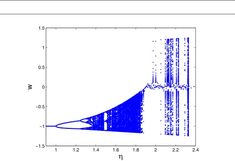
w(k+ 1) =w(k)−ηw5(k) +ηw3(k) (5) where,wis a scalar function, andk≥0, allh> 0. A compact set S ⊂ R is called an invariant set of Function (5), if for any w(0) Î S, the trajectory of Function (5) starting from w(0) will remain in S for all k ≥ 0. Strictly, if 0 <h ≤ 2.32588, then S is an invariant set of Function (5). Especially, if 1 ≤ h ≤ 2.32588, the Douglas’s MCA dynamical system dis-plays the chaotic phenomena illustrated in Figures 1, 2, and 3.
Particularly, some interesting phenomena are shown in Figures 2 and 3, where chaos symmetry and coex-isting are exhibited in the bifurcation diagrams. The key reason of the attractive phenomena is that Equa-tion (5) is an odd funcEqua-tion. If we define w(k) = x, Equation (5) can be rewritten as: If we define w(k) =
1 1.2 1.4 1.6 1.8 2 2.2 2.4
−1.5
−1
−0.5 0 0.5 1 1.5
w
Figure 2Bifurcation diagram of iterative map of Douglas’s MCA algorithmw(0) = 0.7.
1 1.2 1.4 1.6 1.8 2 2.2 2.4
−1.5 −1 −0.5 0 0.5 1 1.5
w
then as
F(−x) = (−x)−η[(−x)5−(−x)3] =−F(x)
Now it is clear that Equation (5) is an odd function. As noted in symmetry in chaos [20], odd function map-ping has a period-doubling cascade, one corresponding to a positive number and the other a negative as the initial point, and the two chaotic attractors spawned by the period-doubling cascades will merge to form one symmetry attractor.
The typical phenomena in the dynamics of symmetric mapping are identified and illustrated by the mathemati-cal model of Equation (5). Specifimathemati-cally, it is observed that, trajectories of attractors from the positive value as their initial condition are shown in Figure 2 and the ones from the negative in Figure 3. Moreover, onh, the chaotic attractors are symmetric if their origins are.
4. STM in chaos control of Douglas’s MCA algorithm
4.1. Dynamics analysis of controlled Douglas’s MCA
algorithm
As is mentioned in Section 2, Jacobian matrix is a powerful approach to judge the non-convergence phe-nomena of dynamical system [24]. A dynamic system is unstable under the condition that each eigenvalue abso-lute of the Jacobian matrix is larger than 1. Lv and Zhang [8] has found that a lot of chaotic behaviors are represented in the interval l Î [1, 2.32588]. Accord-ingly, we use STM to modify the eigenvalue of Jacobian matrix of Equation (5) under the condition and get the
controlled MCA Equation (8) without changing the value and location of unstable fixed points.
From Function (3) and (5)
xk+1=xk+λD[f(xk)−xk]
w(k+ 1) =w(k)−ηw5(k) +ηw3(k))
Hence, the new dynamic equation based on STM method is described as Equation (6):
w(k+ 1) =w(k) +ηλD[w3(k)−w5(k)] (6) when D=I, the controlled MCA Equation (6) is pre-sented as following:
w(k+ 1) =w(k) +λη[w3(k)−w5(k)] (7)
Proof. we define a point w* Î Rn is called an
equili-brium of (7), if and only if
w∗=w∗+λη[(w∗)3−(w∗)5]
Clearly, the set of all equilibrium points of (7) is 0,1, -1.
For each equilibrium, the eigenvalues of Jacobian matrix at this point is computed.
Let
G=w(k) +λη(w3(k)−w5(k))
the Jacobian matrix of (7) is shown as following:
J= dG
dw(k) = 1 +λη(3w 2
(k)−5w4(k))
0 0.5 1 1.5 2
−10 −8 −6 −4 −2 0 2
Lyapunov exponent
There are three cases: As for equilibriumw* = 0
gG
dw(k)|0= 1.
Therefore, 0 is unstable point. As for equilibriumw* = 1
dG
dw(k)|1 = 1−2λη
When0< λ < 1
η, it holds that
dwdG(k)<1. As for equilibriumw* = - 1
dG
dw(k)|−1 = 1−2λη
When0< λ < 1
η, it holds that
dwdG(k)<1. The proof is completed.
Consequently, in the new Jacobian matrix (8) of
Equa-tion (7), each of eigenvalue is less than 1 if0< λ <1
η. In summary, we can control chaotic behavior in the
original system if0< λ <1
η, and the absolute of eigen-value of formula (7) is less than 1 when0< λ <1
η. This means that the dynamic system can converge, and the unstable system is transferred to a stable system by using STM.
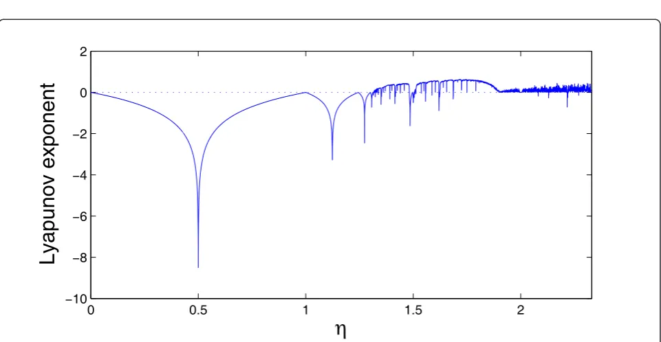
Furthermore, according to the Lyapunov exponent method [19], we can justify and confirm the results by using STM with the illustration of Lyapunov exponent. As mentioned in Section 2.1, when Lyapunov exponent
LE < 0, the system trajectory is stable corresponding to the periodic motion or a fixed point;whenLE > 0, it denotes that the system has dynamic behaviors and pre-sents the chaotic phenomena of strange attractor. The Lyapunov exponent’s transition from negative to positive indicates the change of periodic motion to chaos.
Figures 4 and 5 present the scenarios in which Lyapu-nov exponent of original MCA algorithm and the Lya-punov exponent of the controlled Douglas’s MCA dynamic system by STM separately. In Figure 4, in some intervals of h, the Lyapunov exponent LE is less than 0, while in some intervals, LEis larger than 0 in which the chaotic solutions of MCA algorithm occur. In
0 0.5 1 1.5 2
−0.7
−0.6
−0.5
−0.4
−0.3
−0.2
−0.1 0
Lyapunov exponent
Figure 5Lyapunov exponent of controlled MCA algorithm by STM.
450 455 460 465 470 475 480 485 490 495 500
0.8 0.85 0.9 0.95 1 1.05 1.1
Number of iterations
w
Figure 5, LE < 0 is presented, which means the chaotic behavior of Douglas’s MCA dynamic system has been controlled, and the expected convergent solution of Douglas’s MCA is caught.
4.2. Chaos control of Douglas’s MCA for STM
In this section, case studies of using the STM are illu-strated and the time series results of Douglas’ MCA from different starting points are shown in Figures 6, 7, 8, 9, 10, and 11. For each iterative map w, simulated results of an original system are given to be compared with those using STM. It is evident that the chaotic behaviors of the original dynamic system have been controlled by the STM, the unstable fixed points have been transferred to stable points, and the convergence results have been reached in the original chaotic interval.
Figure 6 illustrates that, whenw = 1.15548,h = 1.3, the original MCA system appears the periodic-4 solu-tions. Moreover, compared with Figures 4 and 6, when
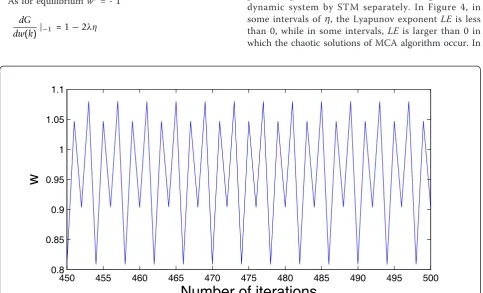
h = 1.3, periodic-4solutions appears clearly. On the other hand, in Figure 4, when h= 1.3, Lyapunov expo-nentLE> 0, periodic oscillate must occur. Concurrently, the absolute of each eigenvalue of the Jacobian matrix J<1. Hence, Lyapunov exponent and the numerical simulation conducted from Jacobian matrix can justify each other. Figure 7 exhibits that whenl= 0.1, the peri-odic oscillation of controlled Douglas’s MCA algorithm by STM is controlled and a convergence solution is achieved.
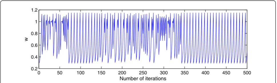
Figure 8 shows whenw= 1.0783, h= 1.93, the origi-nal Douglas’s MCA system appears chaotic solutions. Figure 9 presents that whenl= 0.1, the chaotic beha-vior of Douglas’s MCA algorithm is controlled.
450 455 460 465 470 475 480 485 490 495 500 0.8
0.85 0.9 0.95 1 1.05 1.1
Number of iterations
w
Figure 7Time series of iterative map of controlled Douglas’s MCA algorithm by STMl= 0.1h= 1.3w(0) = 1.15548.
0 1000 2000 3000 4000 5000 6000 7000 8000
0 0.2 0.4 0.6 0.8 1 1.2
Number of iterations
w
Figure 8Time series of iterative mapw(k) of Douglas’s MCA algorithmw(0) = 1.0783h= 1.93.
0 1000 2000 3000 4000 5000 6000 7000 8000 0
0.2 0.4 0.6 0.8 1 1.2
Number of iterations
w
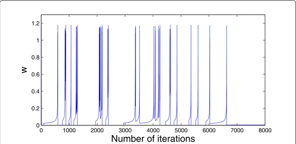
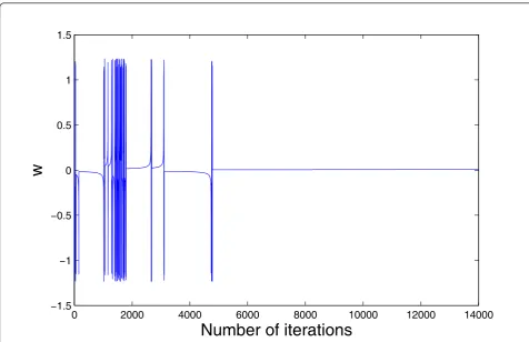
Figure 10 demonstrates that when w= 0.75187, h= 2.25, the original Douglas’s MCA system appears chaos phenomena. Figure 11 describes forl= 0.1, the chaotic behavior of the system is controlled.
In addition, the bifurcation diagrams of Douglas’s MCA algorithm corresponding to different starting pointsw(0) = 0.6 andw(0) = -0.6 are shown in Figures 12 and 13, respectively.
Further, applying the STM to the original MCA sys-tem, the control results of MCA algorithms with respect to Figures 12 and 13 are exhibited in Figures 14 and 15.
It is found that STM can obtain the stable conver-gence solutions of Douglas’s MCA algorithm, and con-trol the numerical instability of periodic oscillation, bifurcation and chaos. Besides, it is worth mentioning that, Figures 12, 13, 14, and 15 also has odd function properties which present symmetric attractors.
5. Conclusion
This article focuses on the chaotic dynamics analysis, and especially chaos control of Douglas’s minor com-ponent analysis algorithm. Periodic oscillation, bifurca-tion, and chaotic behaviors are discussed on the basis of the chaos theory, and the Lyapunov exponent and the Jacobian matrix reflecting the dynamic property of non-linear system are analyzed. Furthermore, the chao-tic phenomena of Douglas’ MCA algorithm under some conditions can be controlled and transformed into a stable system with STM of chaos feedback con-trol, and the convergence solutions can be achieved in the original chaotic intervals. Generally, exploring the chaotic dynamic behavior of Douglas’s MCA is a good path to understand the essential reasons for the non-convergence in MCA method, and it is helpful to extend the effective application of the MCA and related methods.
0 2000 4000 6000 8000 10000 12000 14000
−1.5 −1 −0.5 0 0.5 1 1.5
Number of iterations
w
Figure 10Time series of iterative mapw(k) of Douglas’s MCA algorithmw(0) = 0.75187h= 2.25.
0 2000 4000 6000 8000 10000 12000 14000
−1.5
−1
−0.5 0 0.5 1 1.5
Number of iterations
w
1 1.2 1.4 1.6 1.8 2 2.2 2.4
−1.5
−1
−0.5 0 0.5 1 1.5
w
Figure 12Bifurcation diagram of iterative map of Douglas’s MCA algorithmw(0) = 0.6.
1 1.2 1.4 1.6 1.8 2 2.2 2.4
−1.5
−1
−0.5 0 0.5 1 1.5
w
Moreover, there are lots of non-linear dynamics and chaotic phenomena in real world, a correct and general solution is not easy to achieve. However, the formula-tion of this article proves that STM is a feasible mea-surement to the chaotic behavior control of Douglas’s MCA in the original chaotic interval, and is a novel method to tackle MCA non-convergence issues. Numer-ical results demonstrate that STM is a versatile, effective and simple method to control the instabilities and chaos of MCA algorithm. Future study in the area can be con-ducted to explore the dynamics of other MCA algo-rithms on a wider and deeper level.
Acknowledgements
This study was supported by Applied Basic Research under Grants 2011JY0118.
Author details 1
School of Energy Science and Engineering, University of Electronic Science and Technology of China, Chengdu 611731, P. R. China2School of Mathematics and Computer, Xihua University, Chengdu 610039, P. R. China
Competing interests
The authors declare that they have no competing interests.
Received: 31 August 2011 Accepted: 15 March 2012 Published: 15 March 2012
References
1. DZ Peng, Y Zhang, JC Lv, Y Xiang, A stable MCA learning algorithm. Comput Math Appl.56(4), 847–860 (2008). doi:10.1016/j.camwa.2008.01.016 2. R Klemm, Adaptive airborne mti: An auxiliary channel approach. Proc Inst
Elect Eng.134(3), 269–276 (1987)
3. L Xu, E Oja, Cy Suen, Modified hebbian learning for curve and surface fitting. Neural Netw.5(3), 441–457 (1992). doi:10.1016/0893-6080(92)90006-5 4. K Gao, Mo Ahmad, Mns Swamy, Learning algorithm for total least squares
adaptive signal processing. Electron Lett.28(4), 430–432 (1992). doi:10.1049/ el:19920270
5. S Barbarossa, ED Addio, G Galati, Comparison of optimum and linear prediction techniques for clutter cancellation. Proc Inst Elect Eng.134(3), 277–282 (1987)
6. M George, V Reddy, Development and analysis of a neural network approach to pis-arenko’s harmonic retrieval method. IEEE Trans Signal Process.42(3), 663–667 (1994). doi:10.1109/78.277859
7. Jwr Griffiths, Adaptive array processing, a tutorial. Proc Inst Elect Eng.
130(1), 3–10 (1983)
8. JC Lv, Y Zhang, Some chaotic behaviors in a MCA learning algorithm with a constant learning rate. Chaos Solitions and Fractals.33(3), 1040–1047 (2007). doi:10.1016/j.chaos.2006.01.064
9. Q Zhang, On the discrete-time dynamics of a PCA learning algorithm. Neurocomputing.55(3-4), 761–769 (2003). doi:10.1016/S0925-2312(03)00439-9 10. C Chatterjee, Adaptive algorithm for first principal eigenvector computation.
Neural Netw.18(2), 145–159 (2005). doi:10.1016/j.neunet.2004.11.004 11. PJ Zufiria, On the discrete-time dynamic of the basic hebbian
neural-network nods. IEEE Trans Neural Netw.13(6), 1342–1352 (2002). doi:10.1109/ TNN.2002.805752
12. RC Robinson, An Introduction to Dynamical System: Continuous and Discrete, Pearson Education, New York,
13. DZ Peng, Y Zhang, Convergence analysis of a deterministic discrete time system of feng’s MCA learning algorithm. IEEE Trans Signal Process.54(9), 3626–3632 (2006)
14. JL MaCauley, Chaos Dynamics and Fractals, Cambridge University Press, Cambridge,
15. T Kapitaniak, Controlling Chaos: Theoretical and Practical Methods in Nonlinear Dynamics, Academic, London,
16. JM Vegas, PJ Zufiria, Generalized neural networks for spectral analysis: dynamics and Liapunov functions. Neural Netw.17(2), 233–245 (2004). doi:10.1016/j.neunet.2003.05.001
17. G Dror, M Tsodyks, Chaos in neural networks with dynamical synapses. Neurocomputing.32, 365–370 (2000)
18. E Ott, C Grebogi, JA Yorke, Controlling chaos. Phys Rev Lett.64(11), 1196–1199 (1990). doi:10.1103/PhysRevLett.64.1196
19. A John, An Exploration of Chaos, North-Holland, Amsterdam,
20. M Field, M Golubitsky,Symmetry in Chaos, Society for Industrial and Applied Mathematics (SIAM), Philadelphia, PA, 2
21. D Pingel, P Schmelcher, FK Diakonos, Stability transformation:a tool to solve nonlinear problems. Phys Rep.400(2), 67–148 (2004). doi:10.1016/j. physrep.2004.07.003
22. P Schmelcher, FK Diakonos, Detecting unstable periodic orbits of chaotic dynamical systems. Phys Rev Lett.78(25), 4733–4736 (1997). doi:10.1103/ PhysRevLett.78.4733
23. DX Yang, P Yi, Chaos control of performance measure approach for evaluation of probabilistic constraints. Struct Multidisc Optim.38(1), 83–92 (2009). doi:10.1007/s00158-008-0270-3
24. G Barana, I Tsuda, A new method for computing Lyapunov exponents. Phys Lett A.175(6), 421–427 (1993). doi:10.1016/0375-9601(93)90994-B
doi:10.1186/1687-1499-2012-108
Cite this article as:Zuo and Zhou:Chaos control with STM of minor
component analysis learning algorithm.EURASIP Journal on Wireless Communications and Networking20122012:108.
1 1.2 1.4 1.6 1.8 2 2.2 2.4
Figure 14Bifurcation diagram of iterative map of controlled Douglas’s MCA algorithm by STMw(0) = 0.6.