R E S E A R C H
Open Access
Target guiding self-avoiding random walk
with intersection algorithm for minimum
exposure path problem in wireless sensor
networks
Tinghong Yang
1,2†, Dali Jiang
1*, Haiyang Fang
1†, Mian Tan
1, Li Xie
3and Jing Zhao
2*Abstract
To solve minimum exposure path (MEP) problem in wireless sensor networks more efficiently, this work proposes an algorithm called target guiding self-avoiding random walk with intersection (TGSARWI), which mimics the behavior of a group of random walkers that seek path to their destinations in a strange area. Target guiding leads random walkers move toward their end points, while self-avoiding prevents them from taking roundabout routes. Route intersections further accelerate the speed of seeking connected paths. Dijkstra algorithm (DA) is applied to solve MEP problem in a sub-network formed by multiple connected paths that walkers generate (called TGSARWI DA). Simulations show that the path exposure found by TGSARWI DA is very close to that by DA in the global network (Global DA), whereas the time complexity of computation is much lower. Compared with existing heuristic algorithms such as physarum optimization algorithm (POA), our algorithm shows higher generality and efficiency. This algorithm also exhibits good robustness to the fluctuations of parameters. Our algorithm could be very useful for the solution to MEP problem in fields with large- or high-density sensors.
Keywords:Minimum exposure path, Target guiding, Self-avoiding random walk, Intersection, Time complexity of computation, Robustness
1 Introduction
Wireless sensor network (WSN) is a kind of distributed sensing networks, whose nodes can detect the
surround-ing environment [1–3]. Given the characteristics of
large-scale deployment, easy extensibility, and low price, WSN has been widely applied to such fields as military, target tracking, intelligent transportation, environmental monitoring, and health care [4–11]. The research and application of wireless sensor networks have attracted massive attention.
Coverage is a vital index to evaluate the quality of service (QoS) of WSN’s sensing function [12–16]. According to various characteristics of monitored objects, coverage can
be classified into three types, i.e., area coverage, point coverage, and barrier coverage [17]. The present studies on the measurement of coverage mostly focus on barrier coverage [18–20] and therefore this study on barrier cover-age is aimed to find one or various paths connecting source point and target point, and quantitatively describe the sens-ing quality of mobile objects along the path [21, 22]. The concept of path exposure is used to evaluate coverage qual-ity in the sensor-deployed field with the consideration of path length and exposure simultaneously.
With respect to path exposure, there are two widely diver-gent viewpoints. One is best-case coverage, which is to find a path with the highest observability. The Maximal Expos-ure Path and the Maximal Support Path are two solutions to the best-case coverage [23–25]. The other is the worst-case coverage, which is to design a path through the sensor field and make the minimum probability of detecting the mobile object. There exist two well-known approaches with respect to the worst-case coverage, i.e., minimal exposure
* Correspondence:[email protected];[email protected]
Tinghong Yang and Haiyang Fang contributed equally to this work.
†Equal contributors
1Department of Military Logistics, Army Logistics University, Chongqing, China
2Department of Mathematics, Army Logistics University, Chongqing, China Full list of author information is available at the end of the article
path (MEP) and the maximal breach path [26]. The max-imal exposure path and minmax-imal exposure path are essen-tially the same problem. Hence, we focus on the MEP problem of worst-case coverage in this paper. The MEP problem is the variation of functional extremum in mathem-atics [27]. Theoretically, it is possible to find the optimum path by solving the corresponding Euler-Lagrange Equation [28]. When there is only one sensor in the detecting region, ref. [29] obtains the exact analytical solution to MEP prob-lem. However, in the multiple-sensor region, higher-order non-linearity makes it difficult to express and solve the Euler-Lagrange equation [29–31]. Some approaches have been proposed to address this problem, such as Voronoi diagram-based approach and grid-based approach. However, the time complexity of computation of those approaches will increase with the rise of the grid scale or sensor density. Therefore, it is essential to propose an algorithm to reduce the time complexity of computation and guarantee the qual-ity of solutions simultaneously.
This paper is aimed to decrease the time complexity of computation of grid-based approach in order to solve MEP problem with large-scale field or high-density sensors. An algorithm is proposed and named as target guiding self-avoiding random walk with intersection (TGSARWI), which mimics the behavior that an individual seeks a path from the source point to the target point in a strange area. In this algorithm, multiple random walkers start from the source point and the target point respectively and head to the op-posite sides along edges of the grid network. At each step, each random walker moves to a neighbor chosen according to the edge exposure and the direction to its end point. When routes of walkers from different start points intersect, one or multiple paths will be created between the source and the target, so that a connected sub-network can be formed. Finally, the shortest path algorithm is employed to seek the minimum exposure path in this sub-network.
The main contributions of this paper are summarized as follows:
Compared with the previous algorithm, TGSARWI
DA can solve MEP problem in large-scale field with acceptable complexity.
The complexity of TGSARWI DA is insensitive to
the number of sensors, enabling to solve MEP problem with much higher density sensors.
Unlike the POA, parameters in TGSARWI DA need
no adjustment as the background of MEP problem changes. Hence, the newly proposed algorithm has better adaptability to environment.
The rest of this paper is organized as follows: Section 2 summarizes related approaches about the minimal exposure path problem. Section 3 introduces the model of MEP prob-lem. Section 4 proposes TGSARWI DA algorithm. Section
5 evaluates the proposed TGSARWI DA by extensive simulations.
2 Related work
The goal of MEP problem is to find a path through the detecting region with sensor deployment and to ensure the object that moves along the path has the least possibility detected by sensors. When the detecting region is deployed by multiple sensors, the finding of the minimum exposure path, due to the highly ordered nonlinearity of MEP prob-lem, will become rather complex using the Euler-Lagrange equation. Considering the difficulty in obtaining exact solu-tion to the MEP problem, the most popular strategy is to convert the continuous MEP problem to discrete problem. The discrete method includes two principle approximate ap-proaches. One is Voronoi diagram-based approach and the other is grid-based approach.
Voronoi diagram-based approach is proposed in ref. [26]. In this approach, the detecting region is divided
into n (n is the sensor number) polygons according to
the geometric positions of sensors, and each polygon is called a Voronoi cell. The distance of any point in a Vor-onoi cell to its sensor is closer than that to the other sensors. All the edges of the polygons form a graph called Voronoi graph. The weight of the edge is defined as the exposure along the Voronoi edge. The object can move only along the Voronoi edge. Then, the MEP problem is transformed into a shortest path problem and could be solved by the shortest path algorithm. Many improvements are made based on this approach. For example, Djidjev integrates Voronoi diagram and Euler-Lagrange equation to find the minimum exposure path [29, 30]. Zhang et al. propose a distributed path
search method based on Voronoi diagram [32]. In ref.
[33], Zhou applies Voronoi graph and Dijkstra algorithm to search vulnerable path in the sensors network. How-ever, Voronoi diagram-based approach cannot be used in networks including directional sensors, unless the range of directional sensor is transformed into a special region. In addition, the time complexity of computation will be sharply increased as the total number of sensors grows. Moreover, this approach is also inaccessible when the source and target are not on the Voronoi edges or the sensing intensity is not decided only by the nearest sen-sor [34].
a grid-based approach in the field with directional and omni-directional sensors deployment, and applies the phy-sarum optimization to obtain the minimum exposure path [35]. Ref. [36] proposes a bond percolation-based scheme to put the exposure path problem into a 3D uniform lattice, and then uses grid-based approach to find the minimum ex-posure path. Aiming at the MEP problem with path con-straint conditions, Hao et al. divides the path into three parts. The paths of the first part and the last part are calcu-lated by grid-based approach, while the middle part is solved through the hybrid genetic algorithm [37]. Liu uses adaptive cell decomposition to transform the minimal exposure path problem into a discrete problem, and then designs an OMEPS algorithm to search for the obstacle-avoidance minimum exposure path in the grid-based network [38]. Ac-cordingly, other various improved algorithms based on grid partition also have been proposed [39–42]. It is noted that, in grid-based approach, the larger the scale of the grid net-work within a fixed region is, the more accurate the solution to the MEP problem will be. However, since the complexity rises sharply as the grid scale increases, it is difficult to solve the problem in large-scale grids. Some heuristic algorithms have been proposed to simplify the complexity. For example, Liu et al. proposed a physarum optimization algorithm (POA) based on the light-avoidance of physarum, which could be used to obtain minimum exposure path with edge-cutting method in the grid [40]. The shortage of this method is that, in the simulations, parameters of POA need to be retuned when the grid scale and sensor density change.
3 Minimum exposure path problem
Generally speaking, wireless sensors applied in different fields have different functions, but their common feature is that their detecting sensitivity gradually attenuates as the detecting distance increases. For directional sensor, the sensitivity of the sensor is inversely proportional to the offset angle.
Supposenssensorsfs1;s2;…;snsg, directional or
omni-directional, are randomly distributed in a rectangle field
Q which is an arbitrary point in the sensor-detected
field. The detecting sensitivityss(si,Q) of sensorsito the
pointQcould be represented as follows:
ss sði;QÞ ¼
Where d(si,Q) represents Euclidean distance between
sensorsiand pointQ.V!i denotes the unit vector which determines the sensing direction of sensor siin the case
of directional sensor. siQ! is the vector from sensorsito
pointQ,φðV!i;siQ!Þdenotes the angle between V!i and siQ
!
. Parameter μ, τ, and γ are the sensor-dependent
parameters. According to the literature [40], parameter
μ denotes the sensitivity of the sensor at the unit
distance or the direction of directional sensor, parameter τdenotes the attenuation coefficient of sensor sensitivity
on distance, and parameter γ denotes the attenuation
coefficient of the directed sensor sensitivity on deviating from the central direction.
The sensitivity S of point Q detected by field sensors could be represented by two methods. One is to con-sider the sensitivity S as the sum ofns sensors’
sensitiv-ities, which can be represented asSðQÞ ¼Pns
i¼1ssðsi;QÞ.
The other is to consider the sensitivity S as the
max-imum sensitivity ofnssensors to the pointQ, which isS
ðQÞ ¼ max i¼1;…;nsss
ðsi;QÞ. Following ref. [40], we use the
latter method to represent the sensitivity.
The concept of exposure is used to measure the cover-age quality of the field with sensor deployment. Once the walker’s path f(x) is known, the exposure E(f(x)) of the path could be calculated by curvilinear integral method as follows:
Where vsand veare the source point and target point,
respectively.
MEP problem is to find a path in which the exposure reaches minimum, while the minimum E(f(x)) could be obtained by variation method of extremum. Here, we
denote F¼Sðx;fðxÞÞ
Theoretically, the minimumE(f(x)) can be obtained only when the above equation is solved. However, in the field with multiple sensors, higher-order nonlinearity makes it difficult to solve the Euler-Lagrange equation. Therefore, the problem of continuous minimum exposure path is transformed into a discrete problem in this paper.
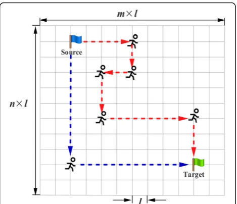
Supposing that the detected field is a rectangle area, the rectangle can be divided intom×ngrids. Then, the walker can move only along the edges of the grid net-work, as shown in Fig.1.
Here, the sensor-detected grid is a weighted connected network graph G= (V,E,W), where V= {v1,v2,…,vi,…,
vm×n} represents the set of all nodes and Eis the set of
all edges. Let wij∈W denote the weight of the edge eij
between two nodesvi andvj, which shows the exposure
of eijdetected by all sensors in the grid field. Since this
Let the length of the edge bel, the coordinate of nodevi
Once the exposure of each edge in the grid is obtained,
the minimum exposure path between source pointvsand
target point ve can be got through optimized algorithm
(such as Dijkstra algorithm). Nevertheless, the time com-plexity of Dijkstra algorithm isO(m2n2), making it difficult to solve MEP problem in a large-scale field. Therefore, this research will apply random walk to imitate the path-finding process of a walker in a strange area. After generating a sufficient number of connected paths between vs and ve,
Dijkstra algorithm is used to seek minimum exposure path in the sub-network formed by these connected paths.
4 TGSARWI DA algorithm for MEP problem 4.1 Self-avoiding random walk
For the random walk algorithm [43], a walker starts at the nodeviand moves to a randomly chosen neighborvj∈V
at each step. The above process could be denoted asxt+ 1 =Pxt, where P represents the matrix of transition prob-ability, which is column-normalized matrix of weighted
adjacency matrix of network graph G. The transition
probability from nodevitovjis inversely proportional to
the weightwijof the edge eij, which could be represented
as follows:
In a random walk, the node-visiting sequence of the walker is a finite state Markov chain, which is only related to the currently visited node rather than the previous sequence of nodes. However, in the shortest path-finding process, the next node that will be visited should not be included in the nodes that have been visited. Namely, the transfer process of MEP problem is not a Markov chain. Thus, a self-avoiding random walk is defined to avoid any visited nodes. In such a random walk, for a path H, the transition probabilitypðij1ÞðHÞfrom nodevitovjis modified
Where, the operator “&” denotes the logical operation symbol “AND”. Unfortunately, as shown in Fig.2, when the walker performs a self-avoiding random walk, it could be besieged by sensors or the previously visited path. In this situation, the walker is expected to take local back-tracking or restart a walk.
4.2 Self-avoiding random walk with intersection
Since the time complexity of computation of the self-avoiding random walk to find a path between a source point and a target point is the square of the distance, the algorithm of self-avoiding random walk with intersection is proposed.
We assume that the source and target are two “bases,” each of which dispatches several“walkers” to contact each
other. When the walkers move in the grid network Gby
self-avoiding random walk, they move by transition prob-abilitypðij1ÞðHÞand leave marks on the nodes that have been visited. If two walkers from two bases meet directly or one walker moves to a node that has been visited by a walker from the opposite base, the path connecting two bases could be generated by routes of these two walkers, as Fig.3 shows. Thus, this process is called as a self-avoiding ran-dom walk with intersection.
Suppose thatnu(nu≫1) walkers are simultaneously
dis-patched from the base vsand ve, respectively, and routes
created by walkers from the two sides are defined asHs ið1
≤i≤nuÞ and Hejð1≤j≤nuÞ. In the seeking process, if Hsi∩ Hej≠∅, there exists one intersection between routes from thei-th walker fromvsand thej-th walker fromve. Then,
these two walkers stop path seeking. Since the walkers Fig. 1The grid network with scalem×n, where the walker can
from the two sides always check the intersection during the seeking processes, they could ensure that the connected path has only one intersection point. The connected path obtained betweenvsandveis described as follows.
Assume thatHsi∩Hej¼ fv0g,Hsi¼ fvs;vi1;vi2;…;vin;v0;
…g, and He
j¼ fve;vj1;vj2;…;vjn0;v0;…g, then the
con-nected path between vs and ve is H¼ fvs;vi1;vi2;…;vin;
v0;vj
n0;vjn0−1;…;vj2;vj1;veg.
4.3 Target guiding self-avoiding random walk with intersection
As a single path obtained by random walk possesses great randomness, it probably includes a roundabout route as
shown in Fig. 3, which is unacceptable as the shortest
path. Thus, target guiding is added in the random walk.
In the algorithm of a random walk with intersection, it is assumed that walkers from each side cannot predict the location of the opposite. In practice, locations of the
base vs and ve could be obtained in advance, so that
walkers from two sides could use the information of their target locations. Then, the algorithm of target
guid-ing self-avoiding random walk with intersection
(TGSARWI) is proposed, whose transition probability is deduced as follows.
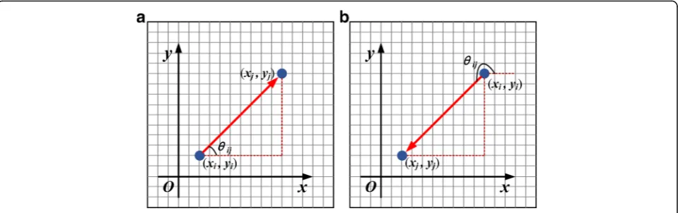
Assuming that the coordinate of each node is
known in the grid network G, and the coordinate of
node vi is (xi,yi). If vi and vj are two nodes in the
network, the ray angle θij from vi to vj is described
as Eq. (7) and Fig. 4.
θij¼
arctan yj−yi
xj−xi
yj−yi
arctan yj−yi
xj−xi
>0
πþ arctan yj−yi
xj−xi
yj−yi
arctan yj−yi
xj−xi
<0 8
> > < > > :
ð7Þ
When a walker whose destination is v∗(x∗,y∗)reaches a
nodevt(xt,yt) through the routeHt, its undirected
transi-tion probabilitypðtj1ÞðHtÞfromvttovjcould be calculated
by Eq. (6). Since locations of vtand vjhave been known
in advance, the transition probability could be
repre-sented by a vectordtj* as follows:
dtj
*
¼pð Þtj1ð ÞHt cosθtj; sinθtj
ð8Þ
Meanwhile, unit vectoret*fromvttov∗is
e*t¼ðcosθt; sinθtÞ ð9Þ
Thus, considering the target guiding, the transition prob-ability can be modified through vector projection as follows: Fig. 3The diagram of self-avoiding random walk with intersection,
where red cycle nodes represent the two bases, the blue and black paths denote the routes walked by walkers from the two bases, respectively. The roundabout path inside the dashed box is unreasonable
pð Þtj2ð Þ ¼Ht dtj
*
e*t¼pð Þtj1ð ÞHt cosθtj−θt ð10Þ
It is noted that the value of transition probabilitypðtj2ÞðHtÞ may be negative. To ensure it satisfies the non-negative and normalization requirement, Eq. (10) is improved as follows:
pð Þtj3ð Þ ¼Ht
pð Þtj1ð ÞHt eρcosðθtj−θtÞ
P
vt;vk ð Þ∈Ep
1
ð Þ
tk ð ÞHt eρcosðθtk−θtÞ
ð11Þ
As is shown above, the transition probability of TGSARWI, whereρ(ρ≥0) is a target guiding factor, repre-sents the strength of target guiding. Whenρ= 0, the target guiding is ineffective, andpðtj3ÞðHtÞ ¼p
ð1Þ
tj ðHtÞ. Whileρ→ +∞, the exposurewtjof the transition edge will play little
role to pðtj3ÞðHtÞ, and the path found by the algorithm is approximately a straight line between the two bases.
4.4 Dijkstra algorithm based on sub-network
Based on random walk algorithm, the TGSARWI algo-rithm would not definitely produce a connected path which is the optimum one. Thus, nh(nh≫1) connected
paths were firstly generated. Then, those paths with the same source point and target point were combined to
construct a connected sub-network G1= (V1,E1,W1) of
the grid network Gfollowed by Dijkstra algorithm (DA)
to solve MEP problem in this sub-network [44].
The exposure value of one path H¼ fvt1;vt2;…;vtpg
is the sum of all edges’ exposures along the path
defined as follows:
E Hð Þ ¼X
p−1
j¼1
wtjtjþ1 ð12Þ
DA is considered as a perfect method to solve the short-est path problem of a single source in a non-negative
weight network. The core idea of DA is that the gener-ation of the new shortest path is based on the existing shortest. Traditional DA has the shortage that it extends only one node by the shortest tentative distance at each
step [45]. In the complex network of grid-based MEP
problem, there is a high probability that multiple nodes have the same shortest tentative distance at one step. Thus, DA is improved to allow the extending of multiple nodes at one step and record necessary information.
Assuming that vs and ve are the source and target
node, respectively, what the researcher needs to do is to find the shortest path between vs and ve. Here,
the weight of edge eij∈E1 is defined as wij in the
sub-network G1. In DA, P and T are denoted as the
sets of permanent and temporary nodes, respectively. Based on the above analysis, the improved DA could be described as follows:
(1) LabelP to the node vs and recordP(vs) = 0. Then,
define the set of new nodes labeledPasR= {vs}. LabelT
to other nodes and record Δ= {vj|vj∈V&vj≠vs}, when ∀vj∈Δ,T(vj) =∞;
(2) For eachvt∈R, for each vj∈Δ&etj∈E1, if T(vj) >
P(vt) +wtj, setT(vj) =P(vt) +wtjandΓ(vj) =vt;
(3) SetR=∅;
(4) For eachvi∈Δ, if TðviÞ ¼ min
vj∈T T
ðvjÞvi≠ve, label P
to the nodevi, and defineP(vi) =T(vi),R=R∪{vi},Δ=Δ −{vi}. ifTðviÞ ¼ min
vj∈Δ T
ðvjÞvi¼ve, labelPto the nodevi,
and defineP(vi) =T(vi), algorithm end, else return to (2).
In the above steps,Γrecords the shortest path informa-tion from the source node to other nodes in the improved DA. The information recorded byΓis incomplete, because the algorithm calculates part of the shortest paths from the source node to all other nodes. However, it can be ensured that the information of the shortest pathHmfrom
vsto ve is complete. Then,Hm can be obtained through
(1)InitializeHm= {Γ(ve),ve} and setvt=Γ(ve); (2)Ifvt=vs, backtracking end, or go to (3); (3)Set Hm ¼ fΓðvtÞg~∪Hm, vt=Γ(vt), and return
to (2).
Where Hmis the shortest path fromvs to ve, which
is an ordered set, ~∪ in step (3) represents ordered
union operation. For example, if there exists an
ordered set A= {v1,v2}, then the following results
will be obtained, fv3g∪~A¼ fv3;v1;v2g and A~∪fv3g
¼ fv1;v2;v3g.
4.5 Algorithm pseudocode
Here, the pseudocode is presented for the overall algorithm, including the TGSARWI algorithm and the improved DA (called TGSARWI DA).
5 Simulation result and discussion
The studies about the convergence and complexity for ran-dom optimization-based heuristic algorithm are usually based on Markov chain, which has no aftereffect property [46–52]. TGSARWI DA is based on the algorithm of self-avoiding random walk and combines target guiding and intersection of paths. Since the walking process does not have after effect property, it no longer belongs to the category of Markov process. Hence, it is inappropriate to do the complexity analysis for our algorithm by common theories. This work integrates theoretical analysis and numerical simulation to discuss the algorithm performance. In this section, simulations are conducted to verify the algorithm for the MEP problem. Firstly, the effect of the parameter ρ on the algorithm is evaluated. Secondly, the algorithm performance is analyzed with precision assess-ment, complexity analysis, and comparison with POA. Finally, the robustness of the algorithm is discussed.
In order to distinguish the application of DA to the glo-bal grid network and the sub-network created by TGSARWI, they are defined as Global DA and TGSARWI DA, respectively.
5.1 Effect evaluation of the target guiding factor
The effects of the target guiding factorρ are discussed on the number of iterations for finding the first connected path (Tf), the number of iterations for finding all the required
connected paths (Tl), and the minimum exposure E(H),
respectively.
The simulation is implemented in the grid with the scale of 50 × 50, in which the length of edge is 10, the number of sensors is 50 and their directions, and coordi-nates are generated randomly. The initial graph created is shown in Fig. 5. For each parameter ρ, the algorithm is simulated 100 times and the average values of Tf,Tl,
andE(H) could be obtained.
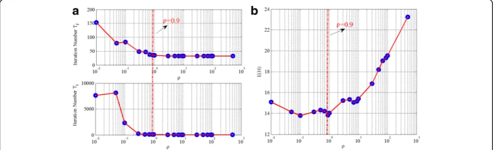
Figure6a shows that when the parameterρ increases,
TfandTldecrease. The reason is that the influence of
tar-get guiding on the transition probability increases with the increment ofρ, which weakens the walker’s randomness and decreases the number of iteration. In fact,TfandTl
de-crease sharply whenρbelongs to the area of [0, 0.9]. How-ever, when ρ> 0.9, the numbers of iterations reach stable. This means that, as ρ further increases, the influence on finding the connected path is little.
The effect of parameterρ to minimum exposureE(H) is displayed in Fig.6b. Roughly speaking, with the increment ofρ, the value of E(H) first decreases and then increases. When ρ is small, the randomness of the walkers is large.
Thus, the sub-network formed by nh connected paths is
E(H) large. Figure 6b shows that E(H) achieves the mini-mum asρ= 0.9. Thus,ρis set as 0.9 in simulations.
Taking ρ as 0.9, the MEP problem presented in Fig.5
is addressed with TGSARWI DA algorithm. It is also solved with Global DA as a comparison. As shown in
Fig. 8, although those algorithms generate different
optimum paths, the values ofE(H) are very close. It is worth to note that TGSARWI DA algorithm owns
good generality. Once the value of parameter ρ is
chosen, the algorithm could solve MEP problem with various field scales and different sensor densities. In the following simulations,ρis always set as 0.9.
5.2 Performance evaluation of TGSARWI DA
The performance of TGSARWI DA algorithm is evalu-ated from three aspects, i.e., precision, complexity ana-lysis, and comparison with POA.
The minimum exposure path found by Global DA is con-sidered as optimal path. Thus, TGSARWI DA is compared with Global DA. Considering the time efficiency, the first path found by TGSARWI is also included in the compari-son. In order to overcome the randomness feature of single simulation, 30 independent repetitive simulations are per-formed and the average value is taken.
The numbers of walkers and connected paths which form sub-network are related with the scale of the field. As for a field with scalem×n, these values are respectively taken as nu¼ b30þp4ffiffiffiffiffiffiffimnc, andnh¼ b30þ2p4ffiffiffiffiffiffiffimnc.
5.2.1 Precision assessment
Since the time complexity of Global DA grows rapidly as field scale increases, simulations are initially conducted in the field whose scale changes from 10 × 10 to 150 × 150 (see Fig.9a). In order to avoid the effect of sensor density, the density of sensors is fixed as 0.02. Namely, the sensor number is 2% of the total number of nodes in the grid net-work. Then, the field scale is fixed as 50 × 50, and the sen-sor density is adjusted from 0.04 to 0.4 (see Fig.9b).
Figure9ashows the trends ofE(H) corresponding to the
first connected path HTFP obtained by TGSARWI, path
HTDAobtained by TGSARWI DA and pathHGDAobtained
by Global DA with the increasing of scale, respectively. E(H) of HTDA andHGDA are almost equal, whose relative error is 4.59% and maximum value is 6.39%. In contrast, E(H) ofHTFPis much larger than that ofHGDA. Their aver-age relative error is 85.49%. In Fig. 9, E(H) of HTDA and HGDAare almost the same in various sensor density fields. In fact, their average relative error is only 2.19%. However, E(H) ofHTFPis greater thanHGDA, and their average rela-tive error is 50.41%. These results suggest that, when deal-ing with MEP problem with various field scales and different sensor densities, TGSARWI DA exhibits perform-ance nearly as well as Global DA.
Fig. 5The initial graph which used to simulate our algorithm, in which sensor types include directional sensor and omnidirectional sensor
5.2.2 Time computation complexity analysis
For a field with scale m×n, the time computation com-plexity of DA is O(m2n2),1which means that DA is not suitable for solving MEP problem with a rather large-scale field. Here, the time computation complexity of Global DA is compared with TGSARWI DA in different grid scales and various sensor densities. The scale of the field is set from 10 × 10 to 900 × 900, and the sensor density is in the area of [0 0.4].
In this paper, the time computation complexity is mea-sured from two aspects, i.e., first connected path found by
TGSARWI and the minimum exposure path found by TGSARWI DA.
For the first connected path, the time computation complexity is mainly associated with the transition pos-sibility pðtj3ÞðHtÞ of each walker at each step in the grid network, which is about O(nu×Tf). Further, the time
computation complexity benefit ηTFP of the first path
found by TGSARWI is defined as the ratio of complexity of finding first connected path by TGSARWI and DA, which is represented as follows:
ηTFP¼
nuTf
mn
ð Þ2 ≈Tf 30ðmnÞ
−2þ
mn
ð Þ−7 4
ð13Þ
For the minimum exposure path, to quantitatively analyze the simplifying efficacy of TGSARWI algorithm
to MEP problem, the reduction ratio ris defined as the
norm ratio of sub-network G1formed by nh connected
paths to the original grid networkG:
r¼‖‖G1‖ G‖ ¼
‖G1‖
mn ð14Þ
Where ‖•‖ is the number of edges of the network.
Since the time computation complexity of sub-network forming is aboutO(nu×Tl), and the time computation
complexity of minimum exposure path found by TGSARWI DA is O(nu×Tl+r2× (m×n)2), the time
computation complexity benefit ηTDA is calculated as
follows:
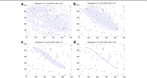
Fig. 7The sub-network created by TGRWI algorithm with different target guiding factor, where theρis set as 0.01, 0.9, 10, and 500, respectively
ηTDA¼
nuTlþr2ðmnÞ2
mn
ð Þ2 ≈Tl 30ðmnÞ−2þ2ðmnÞ−
7 4
þr2
ð15Þ
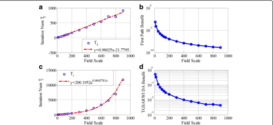
In Fig. 10a, the iteration number Tf is growing
linearly as the field scale increases, whose slope is about 0.9803. Compared with the time computation complexity of DA that is O(m2n2), the efficiency of first path found by TGSARWI algorithm is higher. From Eq. (13) and Fig. 10b, it is shown that the first
path benefit ηTFP decreases significantly as the scale
increases. Specifically, when the field scale is 900 × 900, ηTFP is only 8.3493 × 10⁻⁸. These results suggest that TGSARWI is efficient to find out the first path for timeliness demand in large-scale field, such as real-time solution and online calculation, although
the exposure performance of HTFP is not as good as
Global DA.
In Fig. 10c, although the iteration number Tl of
TGSARWI DA increases exponentially with the change of field scale, its exponential coefficient is only about
0.0046. Meanwhile, in Fig. 10d, the complexity benefit
ηTDA gradually deceases with the increasing of the
scale, and finally goes close to zero. Particularly, its minimum value is 0.0042 when the field has the scale of 900 × 900, suggesting that TGSARWI DA only uses 0.42% computation time of Global DA.
Similar measures are also employed to analyze the time computation complexity of TGSARWI DA with various sensor densities. In Fig. 11a, iteration numbers of the first path found in the field for different sensor densities are visualized. The number of iterations in-creases linearly with the density of sensors in the areas of [0.0.312] and (0.312, 0.4], respectively. The linear re-lation suggests that TGSARWI is not sensitive to the change of sensor density, making it suitable to solve MEP problem in the field with high density sensors.
The equations of the two fitting lines are shown in the inner figure. The slope of the straight line in the latter area is much larger than that in the former area, imply-ing that the time to find a path increases sharply when the density of sensors exceeds the critical value 0.312. This is because if the distribution of sensors is too dense, it will be rather difficult for the walker to find an accessible path. In the area that density of sensors is reasonable (here it is [0, 0.312]), TGSARWI is expected to identify a path at a rather fast speed. For example, when the number of sensors is 780, corresponding to the density of sensor 0.312, only 41 steps are needed to
find the first connected path. Figure11bshows how the
iteration number to find all the required connected paths changes with sensor density. The iteration num-ber Tl is proportional to the sensor density. The curve
increases gently when the sensor density is below 0.312 and grows rapidly as the density is above 0.312. The fit-ting function of the curve is y¼030:4276:2064−x. Accordingly, it is obviously shown that the complexity of finding con-nected path increases as the density becomes denser, while the maximum sensor density for TGSARWI algo-rithm to find connected sub-network is 0.4276.
5.3 Comparison with POA
As a representative of heuristic algorithms in solving MEP problem, physarum optimization algorithm (POA) has the ability to find the minimum exposure path in the field with various type sensors and reduce the time
computation complexity [40]. However, the growth of
time computation complexity is still too fast.
According to ref. [40], in the field with scales of 10 × 10, 20 × 20, 50 × 50, and 100 × 100, as well as with the sensor number of 10, 30, and 50, the minimum expo-sures of paths found by POA and DA are quite close.
The relative errors of E(H) of paths got by POA and
Global DA are 0.0240 and 0.0542 in different field scales and sensor densities. TGSARWI DA is also compared with Global DA in the same condition. The relative errors are 0.0219 and 0.0459 in different field scales and sensor densities, respectively. These results sug-gest that the algorithm has slightly better perform-ance than POA.
The time computation complexity of TGSARWI DA is further compared with that of POA. Numbers of
iteration for POA are taken from ref. [31]. As shown
in Fig. 12, the iteration number of POA is far greater
than that of TGSARWI DA, no matter what scale the field and the sensor density are. These results fully demonstrate that TGSARWI DA is more appropriate to solve MEP problem with a large-scale field and high-sensor density.
5.4 Robustness discussion
In this section, variation coefficient is applied to quantitatively analyze the vulnerability of TGSARWI deceased by the stochastic fluctuations of target
guid-ing factor ρ, the number of walkers nu and the
num-ber of connective paths nh [53]. The fluctuation
coefficient φ(X) of sample data X is defined as:
φð Þ ¼X
ffiffiffiffiffiffiffiffiffiffiffi
D Xð Þ
p
F Xð Þ ð16Þ
where F(X) and D(X) donate the expectation and vari-ance of X, respectively. The closer the coefficientφ(X) to zero is, the smaller fluctuation the sample dataXhas.
Based on current parameters, 100 groups of normal distribution rates are generated and 50 groups of sample Fig. 10The time computation complexity of TGSARWI with various field scales.aShows the trend of iteration number of the first path obtained by TGSARWI.bShows the trend of the first path benefit.cShows the trend of iteration number for finding all the required connected paths.d
Shows the benefit trend of iteration number for finding all the required connected paths
data are created, according to each normal distribution rate. Then, corresponding iteration number Tl, and the
minimum exposure E(H) are calculated according to
each normal distribution. Finally, values of φ(ρ), φ(nu),
φ(nh),φ(Tl), andφ(E(H)) are obtained.φ(Tl) andφ(E(H))
are set as vertical coordinates, φ(ρ), φ(nu), and φ(nh) as
horizontal coordinates, respectively and show their rela-tionships in Fig.13.
From Fig.13a, b,whenρandnufluctuate in the
inter-val [0, 0.5], the fluctuation coefficients of the minimum
exposure E(H) change little, the maximum values of
φ(E(H)) are 0.0331 and 0.0315, respectively. They are all smaller than the corresponding fluctuation coefficients of parameters, indicating that TSAGRWI DA owns quite excellent robustness to the stochastic fluctuations of
these two parameters. In Fig.13c,φ(E(H)) increases qua-dratically with φ(nh), but still satisfies φ(E(H))
<φ(nh).The maximum value of φ(E(H)) is 0.0726,
indi-catingE(H) also owns better robustness to the stochastic fluctuation of nh. In summary, E(H) is not sensitive to
the fluctuation of the three parametersnh,ρ, andnu.
Figure13d–eshow thatφ(Tl) increases as φ(ρ),φ(nu),
and φ(nh) grow. The values of φ(Tl) increases
quadrati-cally with the increase of φ(ρ) and φ(nu), and the
in-creasing rate of the former is faster than the latter. When φ(ρ)≤0.1611 and φ(nu)≤0.2370, the fluctuation
coefficient of Tl is smaller than those of ρ and nu,
sug-gesting thatTlis not sensitive to the fluctuation ofρand
nu in these areas. φ(ρ) > 0.1611 and φ(nu) > 0.2370, the
fluctuation coefficient ofTlis larger than those ofρand
Fig. 12Comparison of time computation complexity for POA and TGSARWI DA with different field scales and sensor number.aShows the comparison of iteration numberTlwith the various field scales.bShows the comparison of iteration numberTlwith the different sensor number
nu, which indicates that Tlis sensitive to the fluctuation
ofρ and nu in these areas.φ(Tl) grows linearly as φ(nh)
increases, and the slope is 0.7224, which is smaller than 1, implying that Tl has better robustness to the
fluctu-ation of nh. In a word, the sensitiveness of iteration
number Tl to the stochastic fluctuations of parameters
could be sorted in descending order asρ,nu, andnh.
It is worth to note that both fluctuation coefficients of TlandE(H) have positive values during the fluctuations of
ρ,nu, andnh, which are mainly caused by the randomness
of TGSARWI.
6 Conclusions
MEP problem comes from the requirement to evaluate the coverage quality of field with sensor deployment. According to the minimum exposure path, the deployment of sensors could be improved. This study aims to enhance the compu-tation efficiency for MEP problem. The random walk is modified from the perspective of target guiding, self-avoiding, and route interaction to propose an algorithm called TGSARWI. A sub-network is constructed by multiple connected paths generated by a group of random walkers using TGSARWI. Then, Dijkstra algorithm is ap-plied to solve MEP problem in this sub-network. The simu-lations mentioned in this study suggest that, the minimum exposure path solved by the approach above is comparable to that solved by Global DA, while the time computation
complexity of TGSARWI DA is only 10−3of that for DA.
Compared with existing heuristic algorithms such as physarum optimization algorithm (POA), this algorithm exhibits higher generality and efficiency. Therefore, our algorithm could solve MEP problem in fields with large-scale or high-density sensors. In fact, it is possible to extend TGSARWI DA to solve the MEP problem in the three-dimensional field, or the field with special protection area, etc. It is expected to shed new lights on the study about MEP problem and promote the development of WSN.
7 Endnotes 1Note
: There also exist some improved Dijkstra’s algo-rithm. For example, the reference [54] uses special data structure, Fibonacci heaps, to improve the efficiency of search and comparison, and then it makes the time com-putation complexity decrease to O(E +VlogV), where E
and V represent the numbers of edge and node in the
graphG(V,E), respectively.
Abbreviations
DA:Dijkstra algorithm; MEP: Minimum exposure path; POA: Physarum optimization algorithm; QoS: Quality of service; TGSARWI: Target guiding self-avoiding random walk with intersection; WSN: Wireless sensor network
Acknowledgements
Not applicable
Funding
This work was partially supported by the National Natural Science Foundation of China under Grant 61372194, Grant 61672038, Grant 70871119, Grant 61502520, Grant 10971227, and Grant 21377166, Excellent Teaching Team Building Project of Logistics Engineering University in 2014, 2110 Engineering Construction Project Phase III, Chongqing Education Reform Project of Graduate under Grant yjg152017, and the Graduate Student Research and Innovation Funding Project of Chongqing in China under Grant CYB16129.
Availability of data and materials
Not applicable
Authors’contributions
In this research paper, D-LJ and JZ devised and guided the research project. T-HY and H.-YF proposed the algorithm. T-HY wrote programs. MT and LX analyzed the results. H-YF wrote the paper. All authors have read and approved the final manuscript.
Authors’information
T.-H.Y. is currently working toward the PhD degree in Institute of Modern Logistics, Logistical Engineering University, China. He received the MS degree in Communication Engineering from Southwest Electronic Telecommunication Research Institute, China, in 2005, and the BS degree in Applied Mathematics from School of science, National University of Defense Technology, China, in 2002. He is an associate professor of Department of Fundamental, Logistical Engineering University, China. His research interests include the fields of Internet of things and multimedia sensor networks.
D.-L.J. received the PhD degree in Traffic management engineering from the School of Transportation and Logistics, Southwest Jiao Tong University, China, in 1998, the MS degree in material flow engineering from Institute of Modern Logistics, Logistical Engineering University, China, in 1990, and the BS degree in automatic control engineering from National University of Defense Technology, China, in 1984. He is a professor and director of Institute of Modern Logistics, Logistical Engineering University, China. He visited University of Missouri at Saint Louis as a research fellow in 2009 and 2010, respectively. His current research include optimization theory and method, logistics and supply chain management, and internet of things, and he has published over 100 papers and seven books on these fields. H.-Y.F. is currently working toward the PhD degree in Institute of Modern Logistics, Logistical Engineering University, China. His research interests include the fields of operational research and optimization theory. M.T. is currently working toward the PhD degree in Institute of Modern Logistics, Logistical Engineering University, China. His research interests include the fields of operational research, complex network and optimization theory.
L.X. received the MS degree in control theory and control engineering from the School of automation, Chongqing University, China, in 2009, and the BS degree in electronic information science and technology from Department of physics and information technology, Chongqing Normal University, China, in 2003. She is an associate professor and director of Department of Information Engineering, Chongqing Electric Power College, China. Her research interests include the fields of Internet of things, electronic information and automatic control. J.Z. received the PhD degree in Biomedical engineering from College of Life Science and Technology, Shanghai Jiao Tong University, China, in 2007, the MS degree in Applied Mathematics from School of Mathematics and Statistics, Chongqing University, China, in 1988. She is a professor and director of Department of Mathematics, Logistical Engineering University, China. Her current research include optimization theory and method, complex network, and network pharmacology, and she has published over 80 papers and five books on these fields.
Competing interests
The authors declare that they have no competing interests.
Publisher’s Note
Author details
1Department of Military Logistics, Army Logistics University, Chongqing, China.2Department of Mathematics, Army Logistics University, Chongqing, China.3Department of Information Engineering, Chongqing Electric Power College, Chongqing 401311, China.
Received: 24 July 2017 Accepted: 19 January 2018
References
1. FL Lewis, Wireless sensor networks. Smart Environments Technologies Protocols & Applications181(1), 11–46 (2016)
2. V Potdar, A Sharif, E Chang, Wireless sensor networks: a survey. Comput. Netw.38(4), 393–422 (2009)
3. P Rawat, KD Singh, H Chaouchi, JM Bonnin, Wireless sensor networks: a survey on recent developments and potential synergies. J. Supercomput.68(1), 1–48 (2014)
4. V Peiris, Highly integrated wireless sensing for body area network applications. SPIE Newsroom., 2–4 (2013)
5. TO Donovan, JO Donoghue, C Sreenan, D Sammorr, PO Reilly, KAO Connor,
A Context Aware Wireless Body Area Network (BAN), Pervasive Computing Technologies for Healthcare Pervasivehealth (2009), pp. 1–8
6. B Liu, Z Yan, MAC CW Chen, Protocol in wireless body area networks for E-health: challenges and a context-aware design. IEEE Wirel. Commun.20(4), 64–72 (2013)
7. JK Hart, K Martinez, Environmental sensor networks: a revolution in the earth system science? Earth Sci. Rev.78(3–4), 177–191 (2006)
8. P Balaya, inSurvey of Energy Harvesting and Energy Scavenging Approaches for on-Site Powering of Wireless Sensor- and Microinstrument-Networks. International Society for Optics and Photonics (California, 2013), p. 87280S 9. A Tiwari, P Ballal, FL Lewis, Energy-efficient wireless sensor network design and implementation for condition-based maintenance. Acm Transactions on Sensor Networks.3(1), 1 (2007)
10. K Saleem, N Fisal, J Al-Muhtadi, Empirical studies of bio-inspired self-organized secure autonomous routing protocol. IEEE Sensors J.14(7), 2232–2239 (2014)
11. G Anastasi, O Farruggia, G Lo Re, M Ortolani,International Conference on System Sciences, Monitoring high-quality wine production using wireless sensor networks (Hawaii, 2009), pp. 1–7
12. J Liang, M Liu, X Kui, A survey of coverage problems in wireless sensor networks. Sensors & Transducers.163(1), 240–246 (2014)
13. D Tao, TY Wu, A survey on barrier coverage problem in directional sensor networks. Sensors Journal IEEE.15(2), 876–885 (2015)
14. C Zhu, C Zheng, L Shu, G Han, A survey on coverage and connectivity issues in wireless sensor networks. Journal of Network & Computer Applications.35(2), 619–632 (2012)
15. A Nayyar, S Sharma, S SAnand Nayyar, A survey on coverage and connectivity issues surrounding wireless sensor network.89 suppl 4(37), 225 (2014)
16. K Hirani, PM Singh, A survey on coverage problem in wireless sensor network. International Journal of Computer Applications.116(2), 1–3 (2015) 17. J CHou, DKY Yau, CYT Ma, Y Yang, H Zhang, IH Hou, NSV Rao,M Shankar,
Coverage in Wireless Sensor Networks. 3(5), 47-79 (2009)
18. S Megerian, F Koushanfar, M Potkonjak, MB Srivastava, Worst and best-case coverage in sensor networks. IEEE Trans. Mob. Comput.4(1), 84–92 (2005) 19. P Balister, B Bollobás, A Sarkar, Barrier coverage. Random Struct. Algoritm.
49(3), 429–478 (2016)
20. Z Wang, J Liao, Q Cao, H Qi, Z Wang, Barrier coverage in hybrid directional sensor networks. IEEE Trans. Mob. Comput.13(7), 1443–1455 (2014) 21. T Clouqueur, V Phipatanasuphorn, P Ramanathan, KK Saluja,In
Proceedings of the 1st ACM international workshop on Wireless sensor networks and applications, Sensor Deployment Strategy for Target Detection (GA, 2003), pp. 42–48
22. L Zhang, X Chen, J Fan, D Wang,Seventh International Symposium on Parallel Architectures, Algorithms and Programming, The Minimal Exposure Path in Mobile Wireless Sensor Network (Nanjing, 2015), pp. 73–79 23. XY Li, PJ Wan, O Frieder, Coverage in wireless ad hoc sensor networks. IEEE
Trans. Comput.52(6), 753–763 (2003)
24. S Megerian, F Koushanfar, G Qu, G Veltri, M Potkonjak, Exposure in wireless sensor networks: theory and practical solutions. Wirel. Netw8(5), 443–454 (2002)
25. J Chang, J Yu, J Ke, J Hu,International Conference on Information NETWORKING and Automation, Simulation of worst and best-case coverage for wireless sensor network (Kunming, 2010), pp. 291–295
26. G Veltri, Q Huang, G Qu, M Potkonjak,International Conference on Embedded Networked Sensor Systems, Minimal and maximal exposure path algorithms for wireless embedded sensor networks (California, 2003), pp. 40–50 27. IM Gelfand, SV Fomin, Calculus of variations. Progress in nonlinear
differential equations and their applications12(3), 141–183 (1963) 28. AH Siddiqui, Applied Functional Analysis. E. Horwood, (1980) 29. HN Djidjev, Approximation algorithms for computing minimum
exposure paths in a sensor field. Acm Transactions on Sensor Networks.
7(3), 23 (2010)
30. HN Djidjev,Third IEEE International Conference of Distributed Computing in Sensor Systems, Efficient computation of minimum exposure paths in a sensor network field (NM, 2007), pp. 295–308
31. L Liu, X Zhang, H Ma,Global Telecommunications Conference, Minimal exposure path algorithms for directional sensor networks (Hawaii, 2009), pp. 6155–6160 32. J Zhou, J Wen, H Zhang, L Zhang, A nodal integration and post-processing
technique based on Voronoi diagram for Galerkin meshless methods. Comput. Methods Appl. Mech. Eng.192(35), 3831–3843 (2003) 33. W Zhang, M Li, W Shu, MY Wu,Second International Conference of Mobile
Ad-hoc and Sensor Networks, Smart Path-Finding with Local Information in a Sensory Field (Hong Kong, 2006), pp. 119–130
34. S Meguerdichian, S Slijepcevic, V Karayan, M Potkonjak,Proceedings of the 2nd ACM International Symposium on Mobile Ad hoc networking and computing, Localized Algorithms in Wireless Ad-Hoc Networks: Location Discovery and Sensor Exposure (New York, 2001), p. 106
35. L Liu, Y Song, H Zhang, H Ma, AV Vasilakos, Physarum optimization: A biology-inspired algorithm for the Steiner tree problem in networks. IEEE Trans. Comput.64(3), 819–832 (2015)
36. X Liu, G Kang, N Zhang, Percolation theory-based exposure-path prevention for 3D-wireless sensor networks coverage. Ksii Transactions on Internet & Information Systems.9(1), 126–148 (2015)
37. H Feng, L Luo, Y Wang, M Ye, R Dong, A novel minimal exposure path problem in wireless sensor networks and its solution algorithm. International Journal of Distributed Sensor Networks.12(8) (2016) 38. L Liu, G Han, H Wang, J Wan, Obstacle-avoidance minimal exposure path
for heterogeneous wireless sensor networks. Ad Hoc Netw.55, 50–61 (2016) 39. L Wang, T Wang, Dynamic heuristic anti-monitoring path searching algorithm
in sensory field. Journal of Computer Applications.28(11), 2767–2770 (2008) 40. L Liu, Y Song, H Ma, X Zhang,INFOCOM of Proceedings IEEE, Physarum
optimization: a biology-inspired algorithm for minimal exposure path problem in wireless sensor networks (Orlando, 2012), pp. 1296–1304 41. M Ye, Y Wang, C Dai, X Wang, A hybrid genetic algorithm for the minimum
exposure path problem of wireless sensor networks based on a numerical functional extreme model. IEEE Trans. Veh. Technol.65, 1–1 (2015) 42. G Kang, X Liu, N Zhang, Y Guo, F Labeau, Critical density for exposure-path
prevention in three-dimensional wireless sensor networks using percolation theory. International Journal of Distributed Sensor Networks.2015(1–12) (2015) 43. F Spitzer, Principles of random walk. J. R. Stat. Soc.73(128), 563 (1964) 44. A DE Knuth, Generalization of Dijkstra’s algorithm. Inf. Process. Lett.6(1), 1–5 (1977) 45. LW Wayne, Operations research: applications and algorithms. Duxbury Press. (1994) 46. G Rudolph, Convergence analysis of canonical genetic algorithms. IEEE
Trans. Neural Netw.5(1), 96–101 (2002)
47. G Rudolph, Finite Markov chain results in evolutionary computation: a tour d’Horizon. Fundamenta Informaticae35(1–4), 67–89 (1998)
48. G Rudolph, inEvolutionary Computation, IEEE World Congress on Computational Intelligence., Proceedings of the First IEEE Conference on 1994. Convergence of non-elitist strategies, vol 61 (1994), pp. 63–66 49. G Rudolph, Convergence of evolutionary algorithms in general search spaces.
IEEE International Conference on. Evolutionary Computation, 50–54 (1996) 50. J He, X Yu, Conditions for the convergence of evolutionary algorithms. J.
Syst. Archit.47(7), 601–612 (2001)
51. G Rudolph, How mutation and selection solve long-path problems in polynomial expected time. Evol. Comput.4(2), 195–205 (2014) 52. Y Yu, ZH Zhou, A new approach to estimating the expected first hitting
time of evolutionary algorithms. Artif. Intell.172(15), 1809–1832 (2008) 53. TS Breusch, AR Pagan, A simple test for heteroscedasticity and random
coefficient variation. Econometrica47(5), 1287–1294 (1979) 54. ML Fredman, Fibonacci heaps and their uses in improved network