Modeling and simulation of air pollutant distribution in street canyon area with Skytrain stations

(1)

R E S E A R C H

Open Access

Modeling and simulation of air pollutant

distribution in street canyon area with

Skytrain stations

Suranath Chomcheon

1,2

_{, Nathnarong Khajohnsaksumeth}

1,2*

_{, Benchawan Wiwatanapataphee}

3

_and

Xiangyu Ge

4

*_{Correspondence:}

nathnarong.kha@mahidol.ac.th

1_{Department of Mathematics,} Mahidol University, Bangkok, Thailand

2_{Centre of Excellence in} Mathematics, Commission on Higher Education (CHE), Bangkok, Thailand

Full list of author information is available at the end of the article

Abstract

This paper focuses on effects of the wind flow velocity on the air flow and the air pollution dispersion in a street canyon with Skytrain. The governing equations of air pollutants and air flow in this study area are the convection–diffusion equations of species concentration and the Reynolds-averaged Navier–Stokes (RANS) equations of compressible turbulent flow, respectively. Finite element method is utilized for the solution of the problem. To investigate the impact of the air flow on the pattern of air pollution dispersion, three speeds of inlet wind in three different blowing directions are chosen. The results illustrate that our model can depict the airflows and dispersion patterns for different wind conditions.

Keywords: Air pollution; Street canyon; Skytrain station

1 Introduction

(2)

numerical models to predict vehicle exhaust dispersion in urban areas with or without a wind field [25]. In his model, the effect of building and street canyon configuration and the turbulent energy produced by moving vehicles on the pollutant propagation were in-vestigated. A few years later in 2014, numerical investigations on pollutant dispersion in street canyons with emission sources located near the ground level were performed by Madalozzo et al. using the pseudo-compressibility hypothesis of mass conservation, the Navier–Stokes equations, energy equation, and pollutant transport equation [26]. Their results show that temperature and street-canyon geometry affect both the wind flow pat-terns and pollutant concentration. Recently, Aristodemou et al. studied the effect of tall buildings on turbulent airflows and pollution dispersion at a seven-building site config-uration using the mesh-adaptive large eddy simulation of incompressible turbulent flow [14]. Suebyat and Pochai investigated numerically air pollution in a heavy traffic area un-der the Skytrain platform in Bangkok, Thailand [27]. Pothiphan et al. studied the impact of wind speeds on heat transfer in a street canyon with a Skytrain station [28]. As the re-sults obtained from existing models are mostly based on incompressible fluid flow with or without the pseudo-compressibility assumption in street canyons with rows of buildings, our understanding of traffic-related air pollution in the street canyon with Skytrain is very limited.

In this study, we investigate the effect of wind velocity on dispersion pattern of the traffic-related air pollution in the street canyon with Skytrain. For a single-pollutant approach to air pollution, namely, carbon dioxide, governing equations of the problem in adiabatic process are the Reynolds-averaged Navier–Stokes (RANS) equations of compressible tur-bulent flow and the convection–diffusion equations of the CO2concentration. Finite ele-ment method is utilized for the solution of the problem. Nine wind conditions are chosen to demonstrate the impact of airflow on the pattern of CO2dispersion in the study region.

2 Mathematical model

To describe the transport of CO2in a street canyon with Skytrain, a transport model for an adiabatic system is developed. The compressible turbulent airﬂow and propagation of CO2 pollutant in the street canton with SkytrainΩ region are governed by the following ini-tial boundary value problem (IBVP) which includes the Reynolds-averaged Navier–Stokes (RANS) equations and the convection–diﬀusion equations of the CO2concentration [29], namely:

• Mass conservation equation of compressible ﬂuid:

∂ρ

∂t +∇ ·(ρu) = 0, (1)

• Reynolds-averaged Navier–Stokes (RANS) equations:

ρ∂u

∂t +ρ(u· ∇)u=∇ ·

–pI+μe

∇u+ (∇u)T

–2

3μe(∇ · u)I – 2 3ρkI

+F, (2)

ρ∂k

∂t +ρ(u· ∇)k=∇ ·

μ+μT σk

∇k+Pk–ρ, (3)

ρ∂ε

∂t +ρ(u· ∇)ε=∇ ·

μ+μT σε

∇ε+Cε1

ε

kPk–Cε2ρ

ε2

(3)

Table 1 Unknown variables

Notation Explanation and unit

ρ density (kg/m3)

u air velocity (m/s)

k turbulent kinetic energy (m2/s2)

ε turbulent dissipation rate (m2_/s3₎ c concentration of carbon dioxide (mol/m3₎

Table 2 Model constants

Constant Value Unit

Cε1 1.44 Cε2 1.92

Cμ 0.09

σk 1.00

σε 1.30

κv 0.41

δw 0.20

κ 1.40

μ 1.509716_×10–5 _(Pa_·_s)

α 0.1592 (m2_/s) uref 1.00 (m/s)

• Pollutant transport equation:

∂c

∂t –∇ ·(α∇c) +u· ∇c=S, (5)

whereρ,u,k,εandcare unknown variables (see the details in Table1),αdenotes diﬀusion coeﬃcient of CO2, andFandSrespectively denote body force and pollution

source, andμeandPkare the eﬀective viscosity and turbulent kinetic energy

production, which are respectively deﬁned by

μe=μ+μt withμt=ρCμk2/ε, and

Pk=μt

∇u:∇u+ (∇u)T.

Other constant model parameters are shown in Table2.

In equation (2),Fcorresponding to body force due to concentration eﬀect is deﬁned by

F=ρβ(c–c0)g, (6)

whereβis the coefficient of volumetric expansion due to concentration variation,gis the gravity acceleration vector, andc0is a reference value for concentration. In adiabatic flow, pressure termp, a function of densityρand the ratio of specific heatκ[30], is defined by

p=1

κρ

κ

. (7)

To completely deﬁne the initial boundary value problem (IVBP), the set of initial and boundary conditions [31] is established as follows:

• The values of CO2concentration at initial statet= 0s is assumed to be zero, i.e.,

(4)

• The pollutant emission sources are from traﬃc vehicles located near the ground level. On the inﬂow boundary of CO2pollutant, we set

c(x,t) =c0, ∀x∈∂ΩS.

• On the inﬂow boundary of turbulent airﬂow∂Ωin, we set

whereuˆ is the unit vector representing wind direction,ITandLTdenote turbulent

length scale and turbulent intensity, respectively, deﬁned by

IT= 0.16Re

• On open (outlet) boundary∂Ωout, the conditions are set to be

• In addition, we apply the near-wall condition on other boundaries∂Ωw, including the

walls of the Skytrain and surrounding buildings, and the surface of the road and the sidewalks, i.e.,

3 Finite element formulation

The variational statement corresponding to the above IBVP is

(5)

= –

Applying the Galerkin approximation, we choose an N-dimensional subspace HN ⊂

H1₍_Ω_{) for}_u_,_ρ_,_k_,_ε_and_H

0⊂H01(Ω) forωu,ωρ,ωk,ωε,ωc. Let{φj}Nj=1 be a set of basis functions ofHN andH0. Then any unknown functionf and test functionhcan be ex-pressed in the following form:

f fN =

Here, we consider a two-dimensional problem. For a 2D linear triangular element, we have a system of nonlinear ordinary diﬀerential equations, fori= 1, 2, 3,

(6)

=1

or in matrix form as

M(e)u˙+ A(e)u= b(e), (26)

whereu˙T_{= (}_ρ_˙_,_u˙_,_k˙_,_ε_˙_,_˙_c₎T_{, u}T_{= (}_ρ_,_u_,_k_,_ε_,_c₎T_{, M}(e) _{and A}(e)_{are the element matrices, and} b(e)_{denotes the load vector deﬁned as follows:}

(7)

b(e)=

By assembling all element matrices and all element vectors, we obtain the global system

Mu˙+ Au = F, (33)

which can be solved by a time integration scheme at any instant of time:

Mun+1– un

t +(un)un= Fn. (34)

(8)

Figure 2Domain mesh

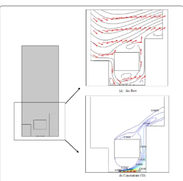
Figure 3Velocity ﬁeld and streamlines of wind and contour lines of CO2concentration obtained from the

(9)

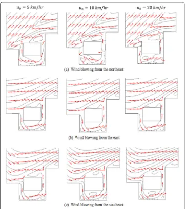
Figure 4Velocity field and streamlines of wind obtained from the model with various features of inlet wind: wind speed of 5 km/h (first column), 10 km/h (second column), and 20 km/h (last column); and the wind blowing towards 3 different directions: (a) northeast; (b) east; (c) southeast

4 Numerical result

This section investigates numerically the effect of the airflow on air pollution dispersion within a street canyon having a Skytrain platform, 20- and 38-meter-tall buildings, and two 5-meter-width sidewalks. COMSOL Multiphysics Modelling software is applied to sim-ulate the finite element approximation of solutions [29]. We assume that no airflow and pollutant emission occur in solid structures including buildings, a Skytrain platform and sidewalks, and emissions of carbon dioxide are only from traffic vehicles under the Sky-train. Figure1presents two-dimensional Skytrain–street-canyon analysis with five emis-sion sources on the ground level. The Skytrain station with width of 21 m and height of 12 m is located 13 m above the traffic level. The computational domain with a nonuniform finite element mesh is shown in Fig.2.

(10)

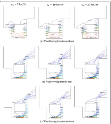
Figure 5Contour lines of CO2concentration obtained from the model with various features of inlet wind:

wind speed of 5 km/h (ﬁrst column), 10 km/h (second column), and 20 km/h (last column); and wind blowing towards 3 diﬀerent directions: (a) northeast; (b) east; (c) southeast

pollutants. Air is assumed to ﬂow into the study region from the left-side rooftop. Figure3

(11)

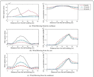
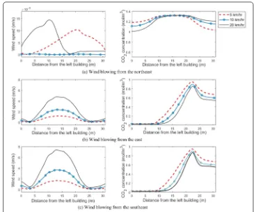
Figure 6Comparison of wind-velocity proﬁles and CO2-concentration proﬁles at 1.5-meter height above the

ground obtained from model with various conditions of the inlet wind speed and its blowing direction

air pollutant concentration obtained from the model with wind blowing from northeast spreads throughout the Skytrain cavity and both sides of the Skytrain station while it dis-tributes to the right-sided region for the inflow wind blowing from east and southeast. Figures6and7compare the profiles of wind velocity and air pollutant concentration at 1.5- and 2-meter heights above the ground obtained from the inflow wind models using 3 different speeds and 3 different wind blowing directions. The results indicate that a lower speed of the inflow wind blowing from both east and southeast gives a higher air pollutant concentration in the Skytrain cavity. It is also found that there is no significant difference of CO2concentration in the Skytrain cavity for different speeds of the inflow wind blowing from the northeast.

5 Conclusion

(12)

Figure 7Comparison of wind-velocity proﬁles and CO2-concentration proﬁles at 2-meter height above the

ground obtained from model with various conditions of the inlet wind speed and its blowing direction

Funding

We would like to thank the Department of Mathematics, Faculty of Science, Mahidol University, and the Center of Excellence in Mathematics, for their ﬁnancial support.

Competing interests

The authors declare that they have no competing interests.

Authors’ contributions

The first author contributed the numerical simulation. The second and third authors formulated a mathematical model, wrote the paper and were responsible for examining results, editing and revising the manuscript. The fourth author verified the analytical methods. All authors read and approved the final manuscript.

Author details

1_{Department of Mathematics, Mahidol University, Bangkok, Thailand.}2_{Centre of Excellence in Mathematics, Commission} on Higher Education (CHE), Bangkok, Thailand.3_{School of Electrical Engineering, Computing and Mathematical Science,} Curtin University, Perth, Australia.4_{Department of Finance, Wuhan Technology and Business University, Wuhan, China.}

Publisher’s Note

Springer Nature remains neutral with regard to jurisdictional claims in published maps and institutional aﬃliations.

Received: 26 July 2019 Accepted: 16 October 2019

References

1. Brunekreef, B., Holgate, S.T.: Air pollution and health. Lancet360(9341), 1233–1242 (2002) 2. Maynard, R.: Key airborne pollutants—the impact on health. Sci. Total Environ.334, 9–13 (2004)

3. Global IGBP change: urban air pollution—a new look at an old problem.http://www.igbp.net/news/features/ features/urbanairpollutionanewlookatanoldproblem.5.19895cﬀ13e9f675e253f0.html

4. Health eﬀects.https://www.airqualitynow.eu/pollution_health_eﬀects.php

5. Sangeetha, A., Amudha, T.: A study on estimation of CO2emission using computational techniques. In: 2016 IEEE International Conference on Advances in Computer Applications (ICACA), pp. 244–249. IEEE, New York (2016) 6. Kongritti, N.: Power-based motor-vehicles model emission of air pollutants from Chalongrat expressway compared to

(13)

7. Is CO2a pollutant?https://skepticalscience.com/co2-pollutant-advanced.htm 8. The eﬀects of carbon dioxide on air pollution.

https://sciencing.com/list-5921485-eﬀects-carbon-dioxide-air-pollution.html

9. The criteria air pollutants.https://en.wikipedia.org/wiki/Criteria_air_pollutants

10. Air pollution.https://www.nationalgeographic.com/environment/global-warming/pollution

11. Abhijith, K.V., Kumar, P., Gallagher, J., McNabola, A., Baldauf, R., Pilla, F., Broderick, B., Sabatino, S.D., Pulvirenti, B.: Air pollution abatement performances of green infrastructure in open-road and built-up street canyon

environments—a review. Atmos. Environ.162, 71–86 (2017)

12. Janhäll, S.: Review on urban vegetation and particle air pollution—deposition and dispersion. Atmos. Environ.105, 130–137 (2015)

13. Rahman, I.A., Putra, J.C.P., Asmi, A.: Modelling of particle transmission in laminar ﬂow using COMSOL Multiphysics. ARPN J. Eng. Appl. Sci.11, 6630–6637 (2006)

14. Aristodemou, E., Boganegra, L.M., Mottet, L., Pavlidis, D., Constantinou, A., Pain, C., Robins, A., ApSimon, H.: How tall buildings aﬀect turbulent air ﬂows and dispersion of pollution within a neighbourhood. Environ. Pollut.233, 782–796 (2018)

15. Baik, J.-J., Kim, J.-J.: A numerical study of ﬂow and pollutant dispersion characteristics in urban street canyons. J. Appl. Meteorol.38(11), 1576–1589 (1999)

16. Chan, T., Dong, G., Leung, C., Cheung, C., Hung, W.: Validation of a two-dimensional pollutant dispersion model in an isolated street canyon. Atmos. Environ.36(5), 861–872 (2002)

17. Chang, C.-H., Lin, J.-S., Cheng, C.-M., Hong, Y.-S.: Numerical simulations and wind tunnel studies of pollutant dispersion in the urban street canyons with diﬀerent height arrangement. J. Mar. Sci. Technol.21(2), 119–126 (2013) 18. Huang, H., Akutsu, Y., Arai, M., Tamura, M.: A two-dimensional air quality model in an urban street canyon: evaluation

and sensitivity analysis. Atmos. Environ.34(5), 689–698 (2000)

19. Ibrahim, A., Altini¸sik, K., Keskin, A.: The pollutant emissions from diesel-engine vehicles and exhaust aftertreatment systems. Clean Technol. Environ. Policy17(1), 15–27 (2015)

20. Kim, J.-J., Baik, J.-J.: A numerical study of thermal eﬀects on ﬂow and pollutant dispersion in urban street canyons. J. Appl. Meteorol.38(9), 1249–1261 (1999)

21. Li, L., Yang, L., Zhang, L.-J., Jiang, Y.: Numerical study on the impact of ground heating and ambient wind speed on ﬂow ﬁelds in street canyons. Adv. Atmos. Sci.29(6), 1227–1237 (2012)

22. Mei, S.-J., Liu, C.-W., Liu, D., Zhao, F.-Y., Wang, H.-Q., Li, X.-H.: Fluid mechanical dispersion of airborne pollutants inside urban street canyons subjecting to multi-component ventilation and unstable thermal stratiﬁcations. Sci. Total Environ.565, 1102–1115 (2016)

23. Miao, Y., Liu, S., Zheng, Y., Wang, S., Li, Y.: Numerical study of traffic pollutant dispersion within different street canyon configurations. Adv. Meteorol.2014, Article ID 458671 (2014)

24. Oyjinda, P., Pochai, N.: Numerical simulation to air pollution emission control near an industrial zone. Adv. Math. Phys. 2017, Article ID 5287132 (2017)

25. Liu, W.: Numerical models for vehicle exhaust dispersion in complex urban areas. Int. J. Numer. Methods Fluids67, 787–804 (2011)

26. Madalozzo, D.M.S., Braun, A.L., Awruch, A.M., Morsch, I.B.: Numerical simulation of pollutant dispersion in street canyons: geometric and thermal eﬀects. Appl. Math. Model.38(24), 5883–5909 (2014)

27. Suebyat, K., Pochai, N.: Numerical simulation for a three-dimensional air pollution measurement model in a heavy traﬃc area under the Bangkok Skytrain platform. Abstr. Appl. Anal.2018, Article ID 9025851 (2018)

28. Pothiphan, S., Khajohnsaksumeth, N., Wiwatanapataphee, B.: Eﬀect of the wind speeds on heat transfer in a street canyon with a Skytrain station. Adv. Diﬀer. Equ.2019, 258 (2019)

29. COMSOL Multiphysics V. 5,Comsol.com. COMSOL AB

30. Poˇrízkovà, P., Kozel, K., Horáˇcek, J.: Numerical solution of compressible and incompressible unsteady ﬂows in channel inspired by vocal tract. J. Comput. Appl. Math.270, 323–329 (2014)