R E S E A R C H
Open Access
Variable bandwidth local maximum
likelihood type estimation for
diffusion processes
Ming T. Tang and Yun Y. Wang
**Correspondence:
School of Science, Jiangxi University of Science and Technology, Ganzhou, People’s Republic of China
Abstract
The method of robust approach is applied to estimate drift function and diffusion function of diffusion processes with discrete-time observations. The proposed method combines the ideas of local linear regression technique and maximum likelihood type estimation technique, so the advantages of local linear estimators persist and overcome the disadvantages of least-squares estimator. Moreover, a variable bandwidth instead of a constant bandwidth is considered in the local maximum likelihood type estimators. The consistency and asymptotic normality of the local maximum likelihood type estimators for drift and diffusion functions are developed under some given conditions. We perform a simulation study to evaluate the robust performances of the proposed estimators.
MSC: 62G35; 62G20
Keywords: Asymptotic normality; Consistency; Robust estimation; Stochastic differential equation; Variable bandwidth
1 Introduction
Diffusion processesXdefined by the following stochastic differential equation are consid-ered in this article:
dXt=μ(Xt)dt+σ(Xt)dBt, (1)
where{Bt,t≥0}is a standard Brownian motion,μ(·) is an unknown measurable function
(drift function) andσ(·) is an unknown positive function (diffusion function). It is well known that diffusion processes driven by Brown motion have been widely used in the fi-nancial and economic fields, and it is often used to model and analyze dynamic changes in asset prices, interest rates, and exchange rates. For example, [1] investigated an appli-cation of Ornstein-Uhlenbeck process to commodity pricing in Thailand. Reference [2] improved estimation of drift parameters of diffusion processes for interest rates by incor-porating information in bond prices. So, recently in the literature, the statistical inference for diffusion processes based on discrete observations has often been of concern; for ex-ample, see [3–6] and its references for parametric estimation, see [7–9] and the references
therein for a semi-parametric estimation and see [10–16] and the references therein for a nonparametric estimation.
As is well known, the first to consider nonparametric estimation for the diffusion co-efficient in model (1) with discrete-time observation was [17], where a kernel type esti-mator was considered. Thereafter, [18] proposed a nonparametric identification and an estimation procedure for the diffusion function after [17], and derived a consistent non-parametric estimator for the drift function by combining their estimator of the diffusion function. Reference [19] constructed the first-, second-, and third-order approximation formulas for drift and diffusion functions by using an infinitesimal generator and Tay-lor expansion. Reference [12] generalized Stanton’s idea and introduced the local polyno-mial estimators for drift and diffusion functions. Since a local linear method may produce negative values for the diffusion function, [14] proposed a new nonparametric estimation procedure of the diffusion function based on re-weighting the Nadaraya–Watson estima-tor.
However, local linear regression methods are very sensitive to outliers, and individual outliers can lead to large changes in the results of statistical inference, therefore lead-ing to irrational and even erroneous conclusions. Such statistical methods like the lo-cal linear regression approach are not strong enough to adapt the complex changing reality, in other words, the local linear regression method is not robust when it comes to outliers or heavy-tailed distributions. In recent years, various robust methods have been proposed for abnormal observation, which has become increasingly crucial and frequent in many research fields. Reference [20] defined maximum likelihood type ro-bust estimates of regression and investigated the asymptotic properties. From then on, the maximum likelihood type robust estimation (M-estimation) has been discussed by many authors, for example, [21, 22] and the references therein. Meanwhile, some mod-ified maximum likelihood type estimators were developed, such as the local maximum likelihood type estimator (local M-estimators), which is a combination of the local lin-ear regression and the M-estimation regression, so the nice properties of local linlin-ear estimator and M-estimator persist. For instance, [23] constructed variable bandwidth local linear M-estimator for a regression function. Reference [24] proposed a nonpara-metric estimator of the regression function by combining local polynomial regression and M-estimation regression. Reference [25] developed robust version of local linear re-gression smoothers for stationary time series sequence. Reference [26] considered local M-estimation of the unknown drift and diffusion functions of integrated diffusion pro-cesses.
The article is organized as follows. The second section constructs the variable band-width local M-estimators of drift and diffusion functions, and the consistency and asymp-totic normality of the new estimators are developed in the same section. Section 3 presents the results of a simulation study. Proofs and auxiliary results are given in Section 4.
2 Local M-estimators and asymptotic theory
Local M-estimation of drift function μ(x) and diffusion function σ2(x) depend on the equations Neglecting the smaller-order terms, the local linear estimator with the variable band-width forμ(x) is defined as the solution to the problem: Choosea1andb1to minimize the weighted sum as
n
and the local linear estimator with the variable bandwidth forσ2(x) is defined as the solu-tion to the problem: Choosea2andb2to minimize the weighted sum as follows:
n tive functions reflecting the variable amount of smoothing at each data point.h/β1(Xi)
andh/β2(Xi) are called variable bandwidth. For more detailed information on variable
bandwidths, see [28–30], among others.
In fact, the aforementioned method used to establish estimators are based on least-squares approach and are not robust. As a result, we choosea1andb1to minimize
n
or to satisfy the following estimation equations:
and
n
i=1 ψ2
(X(i+1)–Xi)2
–a2–b2(Xi–x)
β2(Xi)K
Xi–x
h/β2(Xi)
1
Xi–x
h
=
0 0
, (5)
where ρ1(·) and ρ2(·) are given outlier-resistant functions andψ1(·) and ψ2(·) are the derivatives ofρ1(·) andρ2(·), respectively.
The maximum likelihood type estimators of μ(x) and μ(x) are denoted μˆ(x) =aˆ1 andμˆ(x) =b1, which are the solutions of (4), the maximum likelihood type estimatorsˆ of σ2(x) and (σ2(x)) are denotedσˆ2(x) =a2ˆ and (σˆ2(x))=b2, which are the solutionsˆ of (5).
For a given pointx0, our lemmas and asymptotic theory results are based on the follow-ing conditions.
C 1([10])
(i) The initial conditionX0∈L2and is considered to be independent of{B
t,t≥0}.
(ii) The unknown functionsμ(·)andσ(·)are time-homogeneous and measurable functions onD= (l,u)with–∞ ≤l<u≤ ∞. We also assume the two functions are at least twice continuously differentiable, and satisfy local Lipschitz and growth conditions, that is, for any compact subsetJ⊆D, for allx,y∈J, there exist constantsL1andL2such that
μ(x) –μ(y)+σ(x) –σ(y)≤L1|x–y|,
and
μ(x)+σ(x)≤L21 +|x| .
(iii) σ2(·) > 0onD; (iv) LetS(z) =zz
0exp( y
z0 –2μ(x)
σ2(x) dx)dy,z0∈D, supposeS(z)satisfies
lim
z→lS(z) = –∞, lim
z→uS(z) =∞.
Remark1 The condition C1 ensures the existence and uniqueness of a strong solution to model (1), see [31] for details.
C 2
(i) lus(x)dx<∞, wheres(x) = 2/S(x)σ2(x).
(ii) The initial pointX0has a stationary distributionP0, whereP0is the invariant
Remark2 The conditions C1 and C2 ensure thatXis stationary, and from Kolmogorov forward equation we can get the stationary densityp(x) ofX:
p(x) =us(x)
l s(x)dx
= ξ σ2(x)exp
x
z0 2μ(x) σ2(x)dx
,
wherez0is an arbitrary point insideDandξ is a normalizing constant.
C 3 LetD= (l,u) be the state space ofX, suppose that
lim sup x→u
μ(x) σ(x)–
σ(x) 2
< 0,
lim sup x→l
μ(x) σ(x)–
σ(x) 2
> 0.
Moreover, the mixing coefficient α(k) satisfies k≥1ka(α(k))γ/(2+γ) <∞ for some a> γ/(2 +γ), whereγ is given in the condition C8.
Remark3 The condition C3 guarantees that the processXisα-mixing; see [32] for details.
C 4
(i) The kernel functionK(·)is a continuous probability density function compactly supported on[–1, 1].
(ii) The bandwidthhsatisfiesh→0,nh→ ∞andnh→ ∞asn→ ∞.
C 5 The density functionp(x) of the processXis continuous at the pointx0, andp(x0) > 0. Moreover, the joint density function ofXiandXjis bounded for alli,j.
C 6
(i) minxβ1(x) > 0, andβ1(·)is continuous at the pointx0;
(ii) minxβ2(x) > 0, andβ2(·)is continuous at the pointx0.
C 7
(i) E[ψ1(ui)|Xi=x] =o(1)withui=
X(i+1)–Xi
–μ(Xi);
(ii) E[ψ2(vi)|Xi=x] =o(1)withvi=
(X(i+1)–Xi)2
–σ
2(X
i).
C 8
(i) The functionψ1(·)is continuous and has a derivativeψ1(·)almost everywhere. Additionally, we assume that the following three functions:E[ψ1(ui)|Xi=x],
E[ψ12(ui)|Xi=x],E[ψ12(ui)|Xi=x]are all positive for anyxand continuous at
the pointx0, and there exists a constantγ > 0such thatE[|ψ1(ui)|2+γ|Xi=x],
E[|ψ1(ui)|2+γ|Xi=x]are bounded in a neighborhood ofx0.
(ii) The functionψ2(·)is continuous and has a derivativeψ2(·)almost everywhere. Additionally, we assume that the following three functions:E[ψ2(vi)|Xi=x],
E[ψ22(vi)|Xi=x],E[ψ2 2
(vi)|Xi=x]are all positive for anyxand continuous at
the pointx0, and there exists a constantγ > 0such thatE[|ψ2(vi)|2+γ|Xi=x],
C 9
(i) The functionψ1(·)satisfies
E
sup
|z|≤δ
ψ1(ui+z) –ψ1(ui)|Xi=x
=o(1)
and
Esup
|z|≤δ
ψ1(ui+z) –ψ1(ui) –ψ1(ui)z|Xi=x
=o(δ),
asδ→0uniformly inxin a neighborhood ofx0; (ii) The functionψ2(·)satisfies
E
sup
|z|≤δ
ψ2(vi+z) –ψ2(vi)|Xi=x
=o(1)
and
E
sup
|z|≤δ
ψ2(vi+z) –ψ2(vi) –ψ2(vi)z|Xi=x
=o(δ),
asδ→0uniformly inxin a neighborhood ofx0.
C 10
(i) For anyi,j, suppose that
Eψ12(ui) +ψ12(uj)|Xi=x,Xj=y,
Eψ12(ui) +ψ1 2
(uj)|Xi=x,Xj=y
are bounded in the neighborhood ofx0; (ii) For anyi,j, suppose that
Eψ22(vi) +ψ22(vj)|Xi=x,Xj=y,
Eψ22(vi) +ψ22(vj)|Xi=x,Xj=y
are bounded in the neighborhood ofx0.
Remark4 In fact, the conditions C7–C10 imposed onψ1(·) andψ2(·) are mild and satisfied for many applications, such as Huber’sψ(·) function. For more detailed information on these conditions please refer to [23] or [25].
C 11 Suppose that there exist a sequence of positive integersqnsuch thatqn→ ∞,qn=
o((nh)1/2) and (n/h)1/2α(qn)→0 asn→ ∞.
C 12 Forγ in the condition C8 and allxin a neighborhood ofx0, there existsτ > 2 + γ such that the two functionsE{|ψ1(ui)|τ|Xi=x},E{|ψ2(vi)|τ|Xi=x}are bounded.
C 13 Assumen–γ/4h(2+γ)/τ–1–γ/4=O(1), whereγ is given in the condition C8 andτ is given in the condition C12.
Remark5 The assumptions in condition C3 and C11 on mixing coefficientα(k) is suffi-cient conditions for mixing coeffisuffi-cient, [25] pointed out this assumptions on mixing co-efficient are satisfied given some general conditions. Condition C13 is also satisfied under some weak constraints onγ orτ.
Throughout the whole paper, let
Kl=
We now develop the asymptotic theory for the proposed local M-estimators:
Theorem 1 Under the conditionsC1–C5and the conditions(i)of C6–C10,there exist solutionsμˆ(x0)andμˆ(x0)to equations(4)such that
(ii) Furthermore,if the conditionsC11–C13hold,then
√
(ii) Furthermore,if the conditionsC11–C13hold,then
3 Simulation study
We now perform a Monte Carlo simulation study to evaluate the finite sample perfor-mance of the variable bandwidth local M-estimators by comparing the mean square error (MSE) between them and the Nadaraya–Watson estimators.
We consider the following diffusion processX:
dXt= kernel function, and the bandwidthhis chosen by minimizing the MSE as follows:
1
Throughout the study, we use iterative method to obtainμˆ(·), for any initial valueμˆ0(x), we have
When the following conditions are satisfied, the procedure terminates:
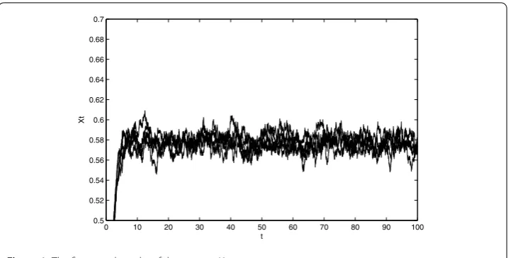
Figure 1 shows the five sample paths of the processXt. Table 1 lists the MSEs of the
Figure 1The five sample paths of the processXt
Table 1 The MSEs of Nadaraya–Watson estimator (MSE1) and variable bandwidth local M-estimator
(MSE2) for drift functionμ(·)
Sample sizen MSE1 MSE2
n= 100 0.0628 0.0667
n= 500 0.0042 0.0036
n= 1000 0.0023 0.0019
n= 5000 0.0014 0.0011
n= 10,000 0.0012 0.0007
indicate that
(i) The MSEs of the two types of estimators decrease toward zero as the sample sizen
increases.
(ii) The variable bandwidth local M-estimator performs better than the Nadaraya–Watson estimator.
4 Lemmas and proofs
The following lemmas are needed to prove the main results of this paper.
Lemma 1 Under the conditionsC1–C5and the conditions(i)of theC6–C10,we have
n
i=1
ψ1(ui)β1(Xi)K
Xi–x0
h/β1(Xi)
(Xi–x0)l
=nhl+1G1(x0) β1l(x0)p(x0)Kl
1 +op(1)
and
n
i=1
ψ1(ui)R1(Xi)β1(Xi)K
Xi–x0
h/β1(Xi)
(Xi–x0)l
=nhl+3 G1(x0) 2βl+2
1 (x0)
μ(x0)p(x0)Kl+2
1 +op(1)
,
Proof of Lemma1 Since the second part of Lemma 1 can be proved by the same arguments as the first one, we only prove the first part. Let
Zn,i=ψ1(ui)β1(Xi)K
Xi–x0 h/β1(Xi)
(Xi–x0)l.
By a change of variable and the continuity at the pointx0ofβ1(·),K(·),G1(·) andp(·), we obtain
E(Zn,1) =
G1(x)β1(x)K
x–x0 h/β1(x)
(x–x0)lp(x)dx
=
G1(x0+yh)β1(x0+yh)Kyβ1(x0+yh)(yh)lp(x0+yh)h dy
=hl+1G1(x0)β1(x0)p(x0)
Kyβ1(x0)yldy1 +o(1)
=hl+1G1(x0) p(x0) β1l(x0)
K(u)uldu1 +o(1)
=hl+1G1(x0)p(x0) βl
1(x0)
Kl1 +o(1).
Therefore, we have
E n
i=1
ψ1(ui)β1(Xi)K
Xi–x0
h/β1(Xi)
(Xi–x0)l
=nhl+1G1(x0) p(x0) β1l(x0)K
l1 +o(1).
Note that
n
i=1 Zn,i=E
n
i=1 Zn,i
+Op
Var
n
i=1 Zn,i
and
Var
n
i=1 Zn,i
=nEZn2,1+ 2
n
j=2
(n–j+ 1)Cov(Zn,1,Zn,j).
By a change of variable and the continuity at the pointx0ofβ1(·),K(·),G3(·) andp(·), we obtain
EZn2,1=
G3(x)β12(x)K2
x–x0 h/β1(x)
(x–x0)2lp(x)dx
=
G3(x0+yh)β12(x0+yh)K2yβ1(x0+yh)(yh)2lp(x0+yh)h dy
=h2l+1G3(x0)β12(x0)p(x0)
K2yβ1(x0)y2ldy1 +o(1)
=h2l+1G3(x0)β11–2l(x0)p(x0)
K2(u)u2ldu1 +o(1)
Letdnbe a sequence of positive integers satisfyingdn→ ∞andhdn→0. Then we have
n
j=2
Cov(Zn,1,Zn,j)= dn
j=2
Cov(Zn,1,Zn,j)+ n
j=dn+1
Cov(Zn,1,Zn,j).
By the conditions C6(i), C10(i) and the bounded support ofK(·), we have
|EZn,iZn,j|
≤E|Zn,iZn,j|
=EEψ1(ui)ψ1(uj)|Xi,Xj β1(Xi)K
Xi–x0
h/β1(Xi)
(Xi–x0)l
×β1(Xj)K
Xj–x0 h/β1(Xj)
(Xj–x0)l
≤C1Eβ1(Xi)K
Xi–x0 h/β1(Xi)
(Xi–x0)lβ1(Xj)K
Xj–x0
h/β1(Xj)
(Xj–x0)l
≤C2h2l+2,
whereC1andC2are constants. Therefore, we have
dn
j=2
Cov(Zn,1,Zn,j)≤C2h2l+2 dn
j=2
1 =onh2l+1.
By using the Davydov inequality, we have Cov(Zn,1,Zn,j)≤C3
α(j– 1)γ/(2+γ)E|Zn,1|2+γ 2/(2+γ)
,
and by the condition C8(i), we have
E|Zn,i|2+γ =E
Eψ1(ui)|Xi β1(Xi)K
Xi–x0 h/β1(Xi)
(Xi–x0)l
2+γ
≤C4Eβ1(Xi)K
Xi–x0
h/β1(Xi)
(Xi–x0)l
2+γ ≤C5h(2+γ)l+1,
whereC3,C4andC5are constants. Therefore, by using the condition C3 and choosingdn
such thatdanhγ/(2+γ)=O(1), we have
n
j=dn+1
Cov(Zn,1,Zn,j)≤C6 n
j=dn+1
α(j– 1) γ/2+γh(2+γ)l+12/(2+γ)
=C6h2l+2/(2+γ)
n
k=dn
α(k)γ/2+γ
≤C6d–nah2l+2/(2+γ)
n
k=dn
whereC6is a constant. In summary, we have
Var
n
i=1 Zn,i
=Onh2l+1.
Therefore,
n
i=1
ψ1(ui)β1(Xi)K
Xi–x0
h/β1(Xi)
(Xi–x0)l=nhl+1
G1(x0) β1l(x0)
p(x0)Kl
1 +op(1)
.
This completes the lemma.
Lemma 2 Under the conditionsC1–C5and the conditions(ii)of C6–C10,we have
n
i=1
ψ2(vi)β2(Xi)K
Xi–x0
h/β2(Xi)
(Xi–x0)l
=nhl+1H1(x0) β2l(x0)p(x0)Kl
1 +op(1)
and
n
i=1
ψ2(vi)R2(Xi)β2(Xi)K
Xi–x0
h/β2(Xi)
(Xi–x0)l
=nhl+3 H1(x0) 2β2l+2(x0)p(x0)
σ2(x0)Kl+2
1 +op(1)
,
where R2(Xi) =σ2(Xi) –σ2(x0) – (σ2(x0))(Xi–x0).
Proof of Lemma2 Using the same techniques in proving Lemma 1, we omit the proof
process.
Lemma 3 Under the conditionsC1–C5, C6–C8(i)andC10(i)–13,we have
1 √
nh
n
i=1ψ1(ui)β1(Xi)K(hX/βi1(–Xx0 i))
n
i=1ψ1(ui)β1(Xi)K(h/Xβi1(–Xxi0
))
Xi–x0
h
D
→N(0,3),
where3=G2(x0)p(x0)β1(x0)V1.
Proof of Lemma3 Let
Wn= n
i=1 Wn,i=
n
i=1
ψ1(ui)β1(Xi)K
Xi–x0
h/β1(Xi)
1
Xi–x0
h
,
then by the condition C7(i), we haveEWn= 0, and
VarWn=Var
n
i=1 Wn,i
=nEWn2,1+ 2
n
j=2
Similar to the proof methods in Lemma 1, we have
VarWn=nhG2(x)p(x0)β1(x0)V1
1 +o(1).
Next, we will show the asymptotic normality of√1
nhWn, and this can be shown by using
similar methods to Theorem 2 of [25]. This completes the lemma.
Lemma 4 Under the conditionsC1–C5, C6–C8(ii)andC10(ii)–13,we have
1 √
nh
n
i=1ψ2(vi)β2(Xi)K(hX/βi2(–Xxi0
))
n
i=1ψ2(vi)β2(Xi)K(hX/βi2(–Xx0 i))
Xi–x0
h
D
→N(0,4),
where4=H2(x0)p(x0)β2(x0)V2.
Proof of Lemma4 The proof methods are similar to those used in Lemma 3.
Proof of Theorem1 (i) We now show that the new robust estimators ofμ(x) andμ(x) are consistent. Let
r= (a1,hb1)T, r0=
μ(x0),hμ(x0) T
,
ri= (r–r0)T
1
Xi–x0
h
,
and
Ln(r) = n
i=1 ρ1
X(i+1)–Xi
–a1–b1(Xi–x0)
β1(Xi)K
Xi–x0
h/β1(Xi)
.
Then we have
ri= (r–r0)T
1
Xi–x0
h
=a1–μ(x0),hb1–hμ(x0)
1
Xi–x0
h
=a1–μ(x0) +hb1–hμ(x0)Xi–x0 h =a1–μ(x0) +b1–μ(x0)(Xi–x0)
=a1+b1(Xi–x0) –μ(x0) –μ(x0)(Xi–x0)
=a1+b1(Xi–x0) +R1(Xi) –μ(Xi)
=a1+b1(Xi–x0) +R1(Xi) –
X(i+1)–Xi
–ui
.
W denote the circle centered atr0and with radiusδbySδ.∀δ> 0, we prove
lim n→∞P
inf r∈Sδ
Ln(r) >Ln(r0)
Forr∈Sδ,
Next, we will show that
where
= –nh
For (9), by the integral mean value theorem, we have
Ln3=
and according to Taylor’s expansion,
∀η> 0, let Dη ={(δ1,δ2, . . . ,δn)T :|δi| ≤η,∀i ≤n}, by the condition C9(i) and |Xi–x0| ≤minxhβ1(x), we get
E
sup Dη
n
i=1
ψ1(δi+ui) –ψ1(ui) –ψ1(ui)δi β1(Xi)K
Xi–x0 h/β1(Xi)
(Xi–x0)l
≤E n
i=1
sup Dη
ψ1(δi+ui) –ψ1(ui) –ψ1(ui)δiβ1(Xi)
×K
Xi–x0
h/β1(Xi)
|Xi–x0|l
≤aηδE
n
i=1
β1(Xi)K
Xi–x0 h/β1(Xi)
|Xi–x0|l
≤bηδ,
whereaη> 0,bη> 0 are two sequences, and satisfyaη→0 andbη→0 asη→0. From
(10) and (11), we can see that
n
i=1
ψ1(zi+ui) –ψ1(ui) –ψ1(ui)zi β1(Xi)K
Xi–x0
h/β1(Xi)
(Xi–x0)l
=op
nhl+1δ,
we get (9) immediately.
LetU1be a positive definite matrix,λbe the smallest eigenvalue of theU1. Accordingly, for anyr∈Sδ,
Ln(r) –Ln(r0)
=Ln1+Ln2+Ln3
=nh
2 G1(x0)p(x0)(r–r0)
TU1(r–r0)1 +o p(1)
+Op
nh3δ
≥nh
2 G1(x0)p(x0)λδ 21 +o
p(1)
+Op
nh3δ.
So asn→ ∞, we have
P
inf r∈Sδ
Ln(r) –Ln(r0) >
nh
2 G1(x0)p(x0)λδ 2> 0
→1,
it follows that (6) holds. In view of (6), one can easily see thatLn(r) has a local minimum in
the interior ofSδ, thus there exist solutions to equation (4). Let (hμˆ(x0),hμˆ(x0))Tdenote
the closest solution tor0= (μ(x0),μ(x0))T, then
lim n→∞P
" ˆ
μ(x0) –μ(x0)2+h2μˆ(x0) –μ(x0)2≤δ2#= 1,
(ii) We derive the asymptotic normality of the new robust estimators ofμ(x) andμ(x).
Then we have
X(i+1)–Xi
=μ(Xi) +ui
=ui+μ(Xi) –μ(x0) –μ(x0)(Xi–x0) +μ(x0) +μ(x0)(Xi–x0)
=ui+R1(Xi) +μˆ(x0) +μˆ(x0)(Xi–x0) +ηˆi–R1(Xi)
=μˆ(x0) +μˆ(x0)(Xi–x0) +ui+ηˆi.
Therefore by (4), we have
=nh
then, by the condition C9(i) and the same argument as that in the first part of Theorem 1, we have
it follows that
√
According to Lemma 3 and the Slutsky theorem, we have
√
Proof of Theorem2 By using Lemma 2 and Lemma 4 instead of Lemma 1 and 3, the proof of this theorem is similar to Theorem 1, so it is omitted here.
5 Conclusions
In this paper, new variable bandwidth nonparametric robust estimators for the drift func-tion and diffusion funcfunc-tion of diffusion processes based on discrete-time observafunc-tions are devised. The new estimators are based on the local linear regression technique and the maximum likelihood type estimation technique, and they have a good control of outliers. The proposed estimators are proved to be consistent and asymptotically normal.
The authors of [23–25] developed robust version estimators of regression function for stationary time series sequence under independent data and dependent data, respectively. Based on their research, in this paper, we studied a continuous-time diffusion process de-termined by a stochastic differential equation, and our robust estimators based on local linear regression techniques; the reader can consider a robust estimator for a diffusion process by using local polynomial regression techniques. Moreover, the basic ideas of this paper have good generality and can be extended to other continuous-time stochastic mod-els.
In addition, in this paper, we only considered robust estimators for the one dimensional diffusion process; in fact, the basic ideas of our methodology hold for the case of multidi-mensional diffusion processes and situations.
Acknowledgements
The authors would like to thank the editor and referees for their valuable suggestions, which improved the structure and the presentation of the paper.
Funding
This research is supported by the NSFC (No.11461032, No.11401267, No.11401169, No.11561028), the Program of Qingjiang Excellent Young Talents, Jiangxi University of Science and Technology, and the NSF of Jiangxi Province (No. 20161BAB211014 and No. 20171BAB201008).
Competing interests
The authors declare that they have no competing interests.
Authors’ contributions
All authors jointly worked on the results and they read and approved the final manuscript.
Publisher’s Note
Springer Nature remains neutral with regard to jurisdictional claims in published maps and institutional affiliations.
Received: 10 August 2017 Accepted: 29 January 2018 References
1. Chaiyapo, N., Phewchean, N.: An application of Ornstein–Uhlenbeck process to commodity pricing in Thailand. Adv. Differ. Equ.2017, 179 (2017)
2. Zou, T., Chen, S.X.: Enhancing estimation for interest rate diffusion models with bond prices. J. Bus. Econ. Stat.35, 486–498 (2017)
3. Tang, C.Y., Chen, S.X.: Parameter estimation and bias correction for diffusion processes. J. Econom.149, 65–81 (2009) 4. Leonenko, N.N., Šuvak, N.: Statistical inference for student diffusion process. Stoch. Anal. Appl.28, 972–1002 (2010) 5. Leonenko, N.N., Šuvak, N.: Statistical inference for reciprocal gamma diffusion process. J. Stat. Plan. Inference140,
30–51 (2010)
6. Li, J., Wu, J.L.: On drift parameter estimation for mean-reversion type stochastic differential equations with discrete observations. Adv. Differ. Equ.2016, 90 (2016)
7. Nishiyama, Y.: Asymptotic theory of semiparametric Z-estimators for stochastic processes with applications to ergodic diffusions and time series. Ann. Stat.37, 3555–3579 (2009)
8. Kristensen, D.: Pseudo-maximum likelihood estimation in two classes of semiparametric diffusion models. J. Econom. 156, 239–259 (2010)
11. Comte, F., Genon-Catalot, V., Rozenholc, Y.: Penalized nonparametric mean square estimation of the coefficients of diffusion processes. Bernoulli13, 514–543 (2007)
12. Fan, J., Zhang, C.: A re-examination of Stanton’s diffusion estimations with applications to financial model validation. J. Am. Stat. Assoc.98, 118–134 (2003)
13. Xu, K.L.: Empirical likelihood-based inference for nonparametric recurrent diffusions. J. Econom.153, 65–82 (2009) 14. Xu, K.L.: Re-weighted functional estimation of diffusion models. Econom. Theory26, 541–563 (2010)
15. Kristensen, D.: Nonparametric filtering of the realized spot volatility: a kernel-based approach. Econom. Theory26, 60–93 (2010)
16. van der Meulen, F., Schauer, M., van Zanten, H.: Reversible jump MCMC for nonparametric drift estimation for diffusion processes. Comput. Stat. Data Anal.71, 615–632 (2014)
17. Florens-Zmirou, D.: On estimating the diffusion coefficient from discrete observations. J. Appl. Probab.30, 790–804 (1993)
18. Jiang, G.J., Knight, J.L.: A nonparametric approach to the estimation of diffusion processes, with an application to a short-term interest rate model. Econom. Theory13, 615–645 (1997)
19. Stanton, R.: A nonparametric model of term structure dynamics and the market price of interest rate risk. J. Finance 52, 1973–2002 (1997)
20. Huber, P.J.: Robust regression: asymptotics, conjectures and Monte Carlo. Ann. Stat.1, 799–821 (1973) 21. Delecroix, M., Hristache, M., Patilea, V.: On semiparametric M-estimation in single-index regression. J. Stat. Plan.
Inference136, 730–769 (2006)
22. Davis, R.A., Knight, K., Liuc, J.: M-estimation for autoregressions with infinite variance. Stoch. Process. Appl.40, 145–180 (1992)
23. Fan, J., Jiang, J.: Variable bandwidth and one-step local M-estimator. Sci. China Math.43, 65–81 (2000) 24. Jiang, J.C., Mack, Y.P.: Robust local polynomial regression for dependent data. Stat. Sin.11, 705–722 (2001) 25. Cai, Z., Ould-Said, E.: Local M-estimator for nonparametric time series. Stat. Probab. Lett.65, 433–449 (2003) 26. Wang, Y.Y., Tang, M.T.: Nonparametric robust function estimation for integrated diffusion processes. J. Nonlinear Sci.
Appl.9, 3048–3065 (2016)
27. Øksendal, B.: Stochastic Differential Equations: An Introduction with Applications. Springer, New York (2005) 28. Fan, J., Gijbels, I.: Variable bandwidth and local linear regression smoothers. Ann. Stat.29, 2008–2036 (1992) 29. Fan, J., Gijbels, I.: Data-driven bandwidth selection in hold polynomial fitting: variable bandwidth and spatial
adaption. J. R. Stat. Soc. B57, 371–394 (1995)
30. Hall, P., Hu, T.C., Marron, J.S.: Improved variable window estimators of probability densities. Ann. Stat.23, 1–10 (1995) 31. Karatzas, I., Shreve, S.: Brownian Motion and Stochastic Calculus. Springer, New York (2012)