R E S E A R C H
Open Access
Wireless indoor network planning for
advanced exposure and installation cost
minimization
Ning Liu
1,2, David Plets
2*, Kris Vanhecke
2, Luc Martens
2and Wout Joseph
2Abstract
The possibility of having information access anytime and anywhere has caused a huge increase of the popularity of wireless networks. Requirements of users and owners have been ever-increasing. However, concerns about the potential health impact of exposure to radio frequency (RF) sources have arisen and are getting accounted for in wireless network planning. In addition to adequate coverage and reduced human exposure, the installation cost of the wireless network is also an important criterion in the planning process. In this paper, a hybrid algorithm is used to optimize indoor wireless network planning while satisfying three demands: maximum coverage, minimal full
installation cost (cabling, cable gutters, drilling holes, labor, etc.), and minimal human exposure. For the first time, wireless indoor networks are being optimized based on these advanced and realistic conditions. The algorithm is investigated for three scenarios and for different configurations. The impact of different exposure requirements and cost scenarios is assessed.
Keywords: Indoor wireless network planning; Optimization algorithm; WiFi (IEEE 802.11n); Coverage; Installation cost and exposure
1 Introduction
Indoor wireless networks are playing a more and more important role in daily life due to the dramatically increas-ing amount of mobile devices. However, an adequate wireless network planning goes beyond providing a cer-tain capacity to the users. A first significant characteristic of the designed network is the installation cost of, e.g., the wireless local area network (WLAN). Whereas current installation cost algorithms mainly look at the number of access points (APs) [1, 2], the full installation cost of a wireless network planning solution includes many more aspects, such as the cabling costs, the costs of drilling holes through walls, and labor costs for getting the APs connected to the power and data network [3]. Secondly, if planning tools account for exposure [4–6] (mostly not, such as [7–9]), they mostly limit or minimize electric-field strengths over the entire simulation area. In real life however, some rooms are more sensitive to high exposure
*Correspondence: david.plets@intec.ugent.be
2Ghent University/iMinds, Dept. of Information Technology, Gaston Crommenlaan 8 box 201, 9050 Gent, Belgium
Full list of author information is available at the end of the article
levels than others. For example, there are usually more people in office rooms than in kitchens or corridors and they also stay there for a longer time. Also, young children are more sensitive to exposure than adults. In daycare or in school buildings, rooms where many young children are present should preferably have lower exposure values. Therefore, this should be accounted for when planning wireless networks.
In this paper, for the first time, a cost optimization is performed that does not only look at merely the access point cost (see [10]) but at the total installation cost, which includes the cost of APs, infrastructure (cable gut-ters, cables, etc.), labor (working hours for installing APs and infrastructure), and other costs which are generated by installing process (such as drilling holes). It has been shown in [11] that the access point cost is only a fraction of the total cost, making the proposed cost optimization the most advanced and realistic one currently available. Furthermore, it is shown how the total human exposure can be minimized from a person-centric view, based on the sensitivity of the rooms to a high exposure value. These sensitivities are determined by the average number
of people present in the rooms and the person types (e.g., children vs. adults). To the authors’ knowledge, this com-bination is now being investigated and realized for the first time. Thirdly, it is shown that also the optimization algo-rithm itself [10] is improved. The remainder of the paper is structured as follows.
In Section 2, related work is presented. Section 3 discusses the wireless configuration and Section 4 the optimization algorithm and the advanced fitness func-tions. In Section 5, three scenarios are introduced and they are simulated and discussed in Section 6. The influ-ence of interferinflu-ence is discussed in Section 6.4. Finally, conclusions are presented in Section 7. Table 1 lists some abbreviations which are used in this paper.
2 Related work
Many researchers have worked on coverage and cost of wireless networks. Some of them focus on decreasing cost by using low-cost components of wireless networks [12, 13], by increasing utilization of equipment [14], or by decreasing energy consumption [15, 16]. However, the complexity of the cost aspect has always been underes-timated, e.g., in [17–19], the number of APs has been used to represent the network planning cost. In [20], the installation cost is accounted for, but it is considered constant and independent of the physical environment, while in reality the installation cost is much more com-plex than that. In [21], the cost of the infrastructure is considered, but the labor costs are ignored. In [22], an
Table 1List of abbreviations
ACO Ant colony optimization
AP Access point
BFS Breadth-first search
CDF Cumulative distribution function
ECP Ethernet connection point
EIRP Equivalent isotropically radiated power
EMF Electromagnetic field
ESL Exposure sensitivity level
GA Genetic algorithm
HIGO Hybrid indoor genetic optimization
IM Interference margin
WLAN Wireless local area network
efficient method for installing telecommunication cabling is presented but with a focus on the relationship of the skill of the cabling work and the installation quality. With respect to human exposure, concerns about the poten-tial health impact of electromagnetic field (EMF) radiation on the human body have arisen [23] and exposure val-ues have been characterized, e.g., in office environments [24, 25]. In [26], it was shown that in indoor environ-ments, exposure values are relevant. In [27], a metric is proposed to assess the environmental impact (e.g., expo-sure) of outdoor networks, but coverage is not accounted for and no (automatic) network planning is performed. In [6], an algorithm was presented to limit or minimize exposure in indoor environments, but it only accounted for coverage and the electric-field strength throughout the building. When the network planner imposes multi-ple requirements (high coverage, low installation cost, and low exposure), more complex optimization algorithms are required. In [28], the network planning problem is solved in radio-frequency identification (RFID) systems by using an altered version of a particle swarm opti-mization (PSO) algorithm. Genetic algorithms (GAs) have been used in [9, 29] for planning wireless communication networks. In [4], coverage and exposure are jointly opti-mized for indoor networks. In [30], a green optimization metric is used, but it is aimed at outdoor cellular base stations. In [31], energy-efficient wireless access networks are designed. However, none of these takes into account the network installation cost, the provided coverage, and an advanced exposure minimization at a same time for indoor wireless networks.
2.1 Comparison of algorithm features with other algorithms
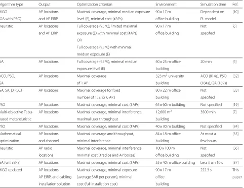
Table 2Overview of features of related wireless network optimization algorithms
Algorithm type Output Optimization criterion Environment Simulation time Ref.
HIGO AP locations Maximal coverage, minimal median exposure 90×17 m Dependent on [10]
(GA with PSO) and AP EIRP level (E), minimal cost (#APs) office building PL model
Heuristic AP locations Full coverage (95 %), limited maximal 90×17 m Not [6]
and AP EIRP exposure (E) with minimal cost (#APs) office building specified
OR
Full coverage (95 %) with minimal
median exposure (E)
GA AP locations Full coverage (95 %), minimal median 40×25 m office 20 min [4]
exposure level (E) building
ACO, PSO, AP locations Maximal coverage 323 m2university ACO (814s), PSO [32]
GA of 1 AP building (184s), GA (189s)
GA, SA, DIRECT AP locations Maximal coverage for fixed 80×22 m office Not [33]
number of 1, 2, or 6 APs building specified
PSO AP locations Maximal coverage, minimal cost (#APs) 64×60 m building Not specified [19]
Multi-objective Tabu- AP locations Maximal coverage, minimal interference, 12,600 m2 3500 min [7]
based metaheuristic maximal user throughput building
PSO AP locations Maximal coverage, minimal cost (#APs) 40×30 m building Not specified [34]
Mathematical AP locations Maximal coverage and throughput, 84×18 m office At most a [35]
optimization and channel minimal interference building few hours
Heuristic AP radio Maximal coverage, minimal interference, 100×100 m Not [36]
locations minimal cost (#radios and AP boxes) office building specified
GA (with BFS) AP locations Maximal coverage, minimal cost (#APs) 55×40 m office building Less than 10 s [37]
HIGO updated AP locations, Maximal coverage, minimal exposure 90×17 m 222.3 s This
AP EIRP, and cabling (average SAR per person), minimal office paper
installation solution cost (full installation cost) building
colony optimization (ACO) algorithm are compared with a GA algorithm for finding the optimal location of 1 AP, where the goal is to only optimize coverage. The paper shows that the PSO and GA algorithm have a compara-ble solution quality and convergence time, while ACO has a significant higher execution time and delivers a slightly worse solution. The work proposed in [33] aims to max-imize the coverage with a given and fixed number of APs (1, 2, 3, or 6) for different optimization algorithms: GA, SA, and DIRECT. DIRECT is based on a division of the design space into hyper-rectangles or hypercubes for multidimensional problems. The paper shows that the algorithms allow improvement of a non-optimized deployment. DIRECT performs well for optimizations with at most 2 APs and GA performs slightly better than SA. In [19, 34], PSO optimizations were performed, able to reduce the number of APs for a given deployment [19] or to design a network with a minimal number of APs [34]. In [7], a Tabu-based metaheuristic optimization algo-rithm is proposed that is focused on QoS, accounting
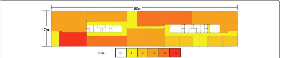
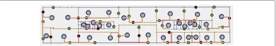
Fig. 1Map of the considered office environment (90×17 m) with indication of the ESL distribution (colorsindicate exposure sensitivity level ESL; the middle rooms (white) have ESL=0)
It will be shown in Section 6.1 that applying an exposure sensitivity level (ESL) distribution indeed significantly influences the network planning and the resulting expo-sure in the considered rooms. Further, when other solu-tions account for the cost, they only aim to minimize the number of installed APs (e.g., previous work in [10]), while it was shown in [11] that this cost is only a fraction of the total cost. The solution presented in this paper therefore takes the entire installation cost into account. Moreover, all calculations are performed within a reasonable time.
3 Configuration
3.1 Simulation environment
Figure 1 shows a map of the considered environment, the third floor of an office building (90×17 m) in Ghent. Coverage and electric-field strength will be evaluated at 425 uniformly distributed receiver locations. These locations are created by overlaying a rectangular grid with a user-defined resolution in the considered office environment. In this paper, the grid size is chosen at 2 m. The locations at which the the IEEE 802.11n APs at 2.4 GHz are installed are chosen from a set of 411 possi-ble uniformly distributed locations on the building floor. These 411 locations are a subset of the 425 locations, since at some of the calculated 425 locations, no AP can be installed (e.g., the room space is too small to install cable and device).
3.2 Coverage model and link budget
The path loss PL (d) [dB] is modeled according to the heuristic model defined in [38, 39]:
PL(d)=PL(d0)+10·n·log10
d d0
+
i
LWi+
j
LBj,
(1)
with PL(d0) [dB] the path loss at a reference distance d0 [ m] (set at 1 m here) according to the distance loss model, d [ m] is the distance along the path between access point and receiver, n [−] is the path loss exponent, iLWi is the cumulated wall loss along
the path, and jLBj is the interaction loss account-ing for propagation direction changes of the path. The model takes into account the effect of the physical envi-ronment on the electromagnetic propagation and bases its calculations on the determination of the dominant path between transmitter and receiver [39]. The electric-field strength is calculated based upon this model, as presented in [6].
The equivalent isotropically radiated power (EIRP) of the access points (802.11n, Section 3.1) will be varied between 0 and 20 dBm by the algorithm, the receiver antenna gain is 0 dBi, and the shadowing margin and fading margin are set at 7 dB (95 %) and 5 dB (99 %), respectively. All networks will be planned for a capacity of 54 Mbps. This corresponds with a required received power of −68 dBm. We select this bit rate and sensitivity to enable us to demonstrate challeng-ing scenarios. Table 3 summarizes the configuration settings.
3.3 Exposure sensitivity levels
An advanced exposure minimization technique will be applied, where different rooms will have different sensi-tivity levels. The ESL of a room is expressed as a number that reflects to which extent high exposure values are considered as adverse. Higher ESL numbers in rooms mean higher sensitivities, i.e., exposure should be lowered (see Fig. 1). This approach will allow designing a network
Table 3Simulation configuration settings of AP (802.11n), receiver, and channel
Items Values
Receiver sensitivity −68 dBm
Receiver antenna gain 0 dBi
Transmitter gain 2 dBi
Frequency 2.4 GHz
AP EIRP range 0−20 dBm
Shadowing margin (95 %) 7 dB
Table 4Unit prices of components contributing to total installation cost
Items Unit price
Cable gutter 13.065e/m
Ethernet cable 1.5e/m
Power cable 4.55e/m
AP 86e
Drilling hole layered drywall 5e
Drilling hole concrete wall 20e
Labor 67.5e/h
Installing APs 2 /h
Installing cables 15 m/h
Drilling holes 5 /h
where in rooms with a high number of people, exposure levels are reduced without impairing coverage. In previ-ous research [6], no differentiation was made between the rooms of a building. Six ESLs are defined in Fig. 1, ranging from 0 to 5. For some rooms, no coverage is required (e.g., sheds, elevator shafts, kitchens,...), since these are rarely visited. These rooms are represented with a white color (ESL=0) in Fig. 1. The five other ESL values (ESL=1 to ESL = 5) are indicated in Fig. 1 with progressively darker colors. The one room with the ESL equal to 5 (bot-tom left in Fig. 1) is a pc room where usually a lot of people are present. The exact ESL of a room is ideally determined by the total absorbed exposure dose of all peo-ple in the different rooms. Besides on the field strength level, this total exposure dose also depends on the average total number of people in each room and the morphol-ogy of these people (adults vs. children). For example, the ESL of the corridor is set at 1, since people mostly walk through this area instead of staying there for a long time. In the following section, it is shown how room ESLs are determined mathematically.
3.3.1 Determination of ESLs
Given the average number of people in each room and their whole-body SAR, each room’s ESL can be derived as
follows. The whole-body SAR of one personpis calculated as SARpwb:
SARpwb=S·SARREF,wb p= E 2
377·SAR REF,p
wb , (2)
withSthe power density andEthe electric-field strength at the person’s location and SARREF,wb pthe reference whole-body SAR of the personp, which is different for adults and children. Since the total SAR of all people in the building is the sum of all SARpwbvalues, Eq. 2 shows that the sum of all reference SARs SARREF,wb pof the people present in a room is a measure for the contribution of that room’sE2to the total SAR of all people in the building. This sum of the SARREF,wb pvalues of personspin a certain room is hereafter called the room’s total reference SAR and is denoted as SARREF,roomwb :
SARREF,roomwb = p=person
in room
SARREF,wb p (3)
Since ESLs are expressed in terms ofE(and SAR is pro-portional to power density or to E2), the square root of the room’s total reference SAR is a measure for the room’s ESL.
ESLroom =
SARREF,roomwb (4)
It can be considered as a good practice to linearly rescale all obtained ESLs to have to lowest non-zero ESL equal to 1. This is done by dividing each ESLroom by the lowest non-zero ESLroomvalue.
3.4 Installation cost
In this paper, for the first time, an indoor planning optimization algorithm is used which accounts for the full installation cost of an indoor environment. Access points only function if they are connected to both a power connection point (PCP) and an ethernet connec-tion point (ECP). Therefore, the total cost of installing the connection cables should also be accounted for. The cost minimization algorithm is based on graph theory and works as described in [11]. The algorithm optimizes the location and the amount of power and ethernet cables that are needed to connect each AP in the considered indoor
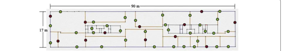
environment to both a PCP and an ECP with the low-est possible cost, based on the algorithm’s input data: the AP,PCP, andECP positions, the cost of cable (ethernet and power) and cable gutter (containing the cables) per meter, drilling holes through walls (material-dependent), and working hours. The number of working hours is determined by the number of holes to be drilled through walls, the number of meters of cables and cable gutters to be installed (dependent on the material of the wall they are attached to), and the number of APs to be installed. It is clear that thephysical layout of the ground planwill greatly influence the output of the algorithm. Table 4 lists the assumed prices of the different cost types. Depend-ing on the amount and location of PCPs and ECPs, the optimal positions of the APs and the total cost will vary. Figure 2 shows a possible set of PCPs and ECPs. The 33 green dots represent the PCPs, and the 12 red dots represent the ECPs.
4 Optimization system
4.1 High-level overview
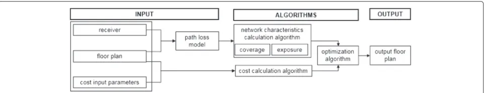
Figure 3 shows a high-level tool chain of the system. A path loss model from the library is applied to the inputted floor plan and chosen receiver. The network characteris-tic calculation algorithm can then, based on these inputs, calculate the coverage and exposure characteristics of a network. Further, the cost calculation algorithm is able to calculate the total installation cost of a network, given the floor plan and the cost input parameters (e.g., the cost per meter cable,...). The optimization algorithm uses the joint outputs of the network characteristic tion algorithm (coverage, exposure) and the cost calcula-tion algorithm (cost) to find an optimal output solucalcula-tion (AP locations, AP transmit power, cabling). The following section will focus on the optimization algorithm itself.
4.2 Optimization algorithm
The optimization algorithm is based on the hybrid indoor genetic optimization (HIGO) algorithm described in [10]. It is a combination of a GA and a quasi-particle swarm optimization (quasi-PSO) algorithm and determines the locations and the EIRP of the APs in the different scenar-ios. Figure 4 shows a flow graph of the algorithm.
In step 1, a starting population of 1000 random solu-tions is generated for the considered environment. In step 2, the scenario’s fitness function is used to calculate the fitness values for all starting solutions. The 40 solutions with the highest fitness values are stored in a first list; the 60 next best solutions in the are stored in a second list. In step 3, 100 crossover solutions are created and evaluated. Offspring solutions are generated by randomly recombining two parent solutions: one from the first list and one from the second list. Due to the smaller size of the first list, solutions in this list have a higher probabil-ity of being selected for recombination than solutions in the second list. In step 4, parts of solutions are changed by the mutation operation by introducing new genetic mate-rial into the population. This basically corresponds with changing the location and/or EIRP of APs of the solution. Within step 4, 50 mutated solutions are created and eval-uated. Compared to [10], the algorithm is improved by a deepened hybrid of the quasi-PSO algorithm: unlike only allowing quasi-PSO for solutions with one AP, all solu-tions can possibly undergo a quasi-PSO operation, with a chance of 25 % (hybrid part). In the mutation phase, a list with the best previous solutions is created for dif-ferent numbers of APs in a solution. If the fitness values of the mutated solution are higher than that of the pre-vious best solution with the same number of APs, the previous solution is replaced by the newly generated solu-tion. Otherwise, a new solution is created according to the following equation (quasi-PSO):
Xi+1=Xi+a(XBest−Xi)+bXR, (5)
with X = location/EIRP, the subscripts “i” and “i+ 1” refer to the previous and the new location/EIRP, respec-tively. The subscript “r” refers to a random location/EIRP. This random location/EIRP is introduced to avoid get-ting stuck in local optima. Subscript “best” refers to the location/EIRP of the nearest AP in the best solution. Parametersaandbare the scaling factors associated with the differences(XBest−Xi)andXR, respectively. Whereas
(XBest −Xi)represents the tendency towards the region of the best location/EIRP,XRintroduces the capability to discover new solutions. Parametersaandbcan be consid-ered as acceleration constants. The higher theaandb, the
Fig. 4Flow graph of evaluation process of a proposed solution
higher the acceleration towards the current best position and the random position, respectively. In this paper, they are both equal to 0.4. After step 4, a new iteration from step 2 is started by resorting the first and second list based on their fitness value. In this paper and for the considered environment, the algorithm is stopped after 100 executed iterations of steps 2, 3, and 4. In the next section, it is explained how a proposed solution is evaluated (“solution evaluation” block in Fig. 4).
4.3 Solution evaluation
Each solution that is proposed by the optimization algorithm, whether being randomly generated or by a crossover or mutation operation, consists of a set APs, each with a specific location and EIRP. As shown in Fig. 5, together with the fitness function that is considered for the scenario, this set of APs serves as an input to the solu-tion evaluasolu-tion module of the algorithm. Based on the phyiscal properties (walls, dimensions,...) of the floor plan,
the location and EIRP of the APs, the location of the DCPs and ECPs, the type of receiver, the path loss model, and the cost input parameters, the network calculator predicts the output characteristics of the wireless network. This comprises the coverage and field strength value in each receiver point and the total installation cost of the wireless network. Using the proposed fitness function, this output allows an evaluation of the fitness function value. In the next section, the building blocks for the fitness functions will be discussed: coverage fitness, installation cost fitness, and exposure fitness based on ESLs.
4.4 Coverage fitness
The first fitness functionf1 evaluates the coverage for a certain literature capacity of a certain solution and will often be the most important requirement.
f1=100fcov ftot
(6)
Fig. 6The normal connection point distribution (green= power,red= ethernet) and the considered solution with cost costmax(purple dots represent APs, EIRP is shown insidedot)
wherefcovis the number of receiver points covered by the wireless network andftot is the total number of receiver points requiring coverage.f1will have a value between 0 and 100.
4.5 Installation cost fitness
As indicated in Section 3.4, different network deploy-ments may correspond with largely different installation costs.f2represents the installation cost fitness:
f2=100 costtotal costmax
. (7)
costtotalrepresents the total installation cost of the consid-ered network design. However, to evaluate the fitness, it should be set out against a reference maximal cost costmax. As costmax, the installation cost of the network in Fig. 6 is assumed, in which 32 APs are installed, one or two in each of the larger rooms, zero in the very small rooms. The light green lines represent the power cables, and the red lines represent the ethernet cables. For this configu-ration, costmaxequalse10312.f2will, for all deployments here considered, have a value between 0 and 100.
4.6 Exposure fitness
Two exposure fitness functions are defined. The calcu-lation of the first exposure fitness function, f3, is based on the electric-field strength observed at the receiver locations, and on the ESLs of the rooms:
f3=100 E ESL 50
EESL50max, (8)
with EESL50 the median of the electric-field strengths (in V/m) at the different receiver locations. The ESL of the
room of the receiver location is accounted for by giving locations in high ESL rooms more weight: an electric-field strengthEat a receiver location inside a room with ESL=i (i=0..5) is addeditimes to the cumulative distribution function (CDF) of the field strengths. For example, an electric-field strengthE=0.1 V/m in the corridor in Fig. 1 (ESL=1) contributes to the global cdf with one 0.1 V/m value, while an electric-field strengthE=0.4 V/m in the top left room in Fig. 1 (ESL=3) contributes to the global CDF with three 0.4 V/m values.EESL50maxis defined asEESL50 for a configuration with maximal electric-field strengths (all 411 APs are active with an EIRP value of 20 dBm). Whereas the first exposure fitness function assesses the median field values, the second one, f4, also represents the spatial homogeneity (i.e., absence of large spatial vari-ations) of the field strengths, by minimizing the maximal (95th percentiles) field values instead of the median field values inf3:
f4=100 E ESL 95
EESL95max, (9)
where EESL95 andE95maxESL are defined asEESL50 andEESL50max, respectively, but for the 95 % percentile instead of for the 50 % percentile. TheE50maxESL (in Eq. 8) andE95maxESL (in Eq. 9) values are 10.95 and 59 V/m, respectively, for this envi-ronment. For all deployments here considered, f3andf4 will have a value between 0 and 100. By weighing the field strengths with the room’s ESL, the exposure minimization algorithm advances current methods by enabling mini-mization of specific rooms that are sensitive to a higher exposure.
Fig. 8Network layout for scenario I with indication of ESL distribution (purple dot= AP with EIRP indicated insidedot,colorsinside rooms (see legend) indicate ESL).aFirst ESL distribution.bSecond ESL distribution
4.7 Combined fitness function
Combination of the four presented fitness functions in a global fitness functionf5allows optimizing networks that are subject to multiple requirements:
f5=w1f1−w2f2−w3f3−w4f4. (10)
Depending on the specific aim of the network design, the value of the weightswi (i=1..4) can be determined. The optimal solution is the one with the highest fitness function (f5) value, as it corresponds to the highest cover-age percentcover-age, the lowest total installation cost, and the lowest exposure values.
5 Scenarios
In this section, three scenarios are defined to investigate the impact of coverage (required bit rate of 54 Mbps), installation cost, and human exposure requirements on the network planning of the office environment in Fig. 1. The specific network requirements will determine the fitness functions that will be used in the optimization algorithm.
5.1 Scenario I: maximal coverage with minimal human exposure
Scenario I intends to obtain a coverage rate of 100 % for a capacity of 54 Mbps with a minimal median exposure and a high spatial homogeneity. The weight factors,w3andw4 in Eq. 10, need to be a positive number. In this way, the algorithm will obtain a solution with a low exposure level, in order to achieve 100 % coverage at 54 Mbps. This yields the following fitness functionf5(see Eq. 10):
f5=1×f1−0.1×f3−0.1×f4, (11)
The values ofw3andw4are chosen at 0.1, making the total exposure weight equal to 0.2.w1is set at 1 to make the coverage fitness dominant over the exposure fitness and obtain a solution with 100 % coverage for a capacity of 54 Mbps. This scenario will be tested for two differ-ent ESL distributions. The first ESL distribution is the one displayed in Fig. 1. In order to assess the influence of the ESL distributions, a second ESL distribution is defined, which is the reversed version of the first one: rooms with ESL = 1, 2, 3, 4, 5, according to the first ESL distribu-tion, have ESL=5, 4, 3, 2, and 1, respectively, according to the second ESL distribution. This will allow assessing the influence of the ESL distribution on the field values in rooms with different ESLs and on the resulting network planning layout.
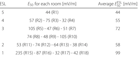
Table 5Median field valuesE50per room for the first ESL distribution (Fig. 8) (Ri,i=1..18 represents room numberi)
ESL E50for each room [mV/m] AverageEESL50 [mV/m]
5 44 (R1) 44
4 57 (R2) - 75 (R3) - 32 (R4) 55
3 105 (R5) - 47 (R6) - 51 (R7) 72
74 (R8) - 48 (R9) - 105 (R10)
2 53 (R11) - 74 (R12) - 64 (R13) - 38 (R14) 58
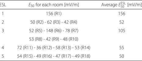
Table 6Median field valuesE50per room for the second ESL distribution (Fig. 8) (Ri,i= 1..18 represents room numberi)
ESL E50for each room [mV/m] AverageE50ESL[mV/m]
1 156 (R1) 156
5.2 Scenario II: maximal coverage with minimal installation cost
Scenario II aims to obtain a solution with a coverage rate of 100 % for a capacity of 54 Mbps and a minimal installa-tion cost.w2for scenario II is chosen based on the similar principle to that of scenario I. This yields the following fitness functionf5:
f5=1×f1−0.2×f2. (12)
The value ofw2is chosen at 0.2 here, making the cov-erage fitness (w1=1) dominant over the installation cost fitness and again obtain a solution with 100 % coverage for a capacity of 54 Mbps. This scenario will be tested for two different configurations: one with the set of connection points (CPs) as in Figs. 2 and 6, and one with a reduced set of possible connection points, as displayed in Fig. 7. This will allow assessing the influence of the size of the con-nection point set on the total installation cost and on the resulting network planning layout.
5.3 Scenario III: maximal coverage with minimal human exposure and minimal installation cost
Scenario III intends to obtain a coverage rate of 100 % for a capacity of 54 Mbps with a minimal installation cost, minimal median exposure values, and a high spa-tial homogeneity of the field values. As for weight factors off5, the ratio of weight factors (w1,w2,w3, andw4) can be adapted based on the different requirements, which generate solutions with the different characteristics. The influence of weight factors are similar with those of in [10]. In scenario III, fixed weight values are considered. This yields the following fitness functionf5:
f5=1×f1−0.2×f2−0.1×f3−0.1×f4. (13)
Table 7Performance of old algorithm and new improved algorithm
Algorithm Coverage [%]EESL50 [mV/m]E95ESL[mV/m] Simulation time [s]
Old algorithm 100 47.8 146.4 215.5
New algorithm 100 46.5 132.4 222.3
The value ofw2is again chosen at 0.2 here, making the installation cost fitness of equal importance as the total exposure fitness (w3 = w4 = 0.1). The coverage fitness (w1 = 1) is still dominant over the installation cost and exposure fitness, yielding optimal solutions with 100 % coverage for a capacity of 54 Mbps. This scenario will be executed for the ESL distribution shown in Fig. 1 and for the two different connection point distributions presented in Section 5.2. It should be noted that for all scenarios, the ratio of the weights w1 andw2, w3, andw4 is large enough to ensure a coverage percentage of (nearly) 100 %. A drastic reduction of this ratio would lead to results that are suboptimal for the goal of this optimization (cover-age percent(cover-age below, e.g., 95 % or worse). In general, a high importance of a low median and 95 % percentile exposure (high values for w3 and w4, respectively) will lead to wireless deployments with smaller coverage per-centages and higher installation cost, which can be coun-tered by increasing w1 andw2, respectively. Depending on the deemed importance of each specific optimization goal (coverage, cost, median exposure, maximal expo-sure), the value of the weights can be freely adjusted to favor the achievement of one or more (possibly conflicting) goals.
6 Results
This section analyzes the characteristics of the optimized wireless networks, according to the scenarios defined in Section 5. It should be noted that all network layouts that will be presented hereafter correspond to a coverage rate of 100 % for a capacity of 54 Mbps. This is due to givingf1 a higher weight than the other fitness components (f2,f3, andf4) in all three scenarios.
6.1 Scenario I: maximal coverage with minimal human exposure
Figure 8a and 8b shows the optimal layout of the network designed in scenario I for the first and second ESL distri-bution, respectively. The locations of the APs are indicated with purple dots and their EIRP with a value inside the purple dot. The figures show that in both cases, access points are preferably placed in rooms with low ESL values, as could be expected.
Fig. 9Resulting network layout for scenario II with indication of cabling (red dot/line=ethernet CP/cable,green dot/line=power CP/cable,purple dot=AP with EIRP indicated insidedot).aNormal set of connection points.bReduced set of connection points
ESL = 1 vs. 44 V/m for ESL = 5 for the first ESL distribu-tion and 156 mV/m for ESL = 1 vs. 50 V/m for ESL = 5 for the second ESL distribution. Indeed, reversal of the ESL distributions leads to significant changes in median expo-sure levels: the average median expoexpo-sure level for room 1 for the second ESL distribution (ESL = 1) (156 mV/m) is 255 % larger than for the first ESL distribution (ESL = 5) (44 mV/m). Analogously, for rooms 15–18, the average median exposure level for the second ESL distri-bution (ESL = 5) (50 mV/m) is 49 % less than for the first ESL distribution (ESL = 1) (99 mV/m). The results indi-cate the benefits of introducing the ESL distributions for advanced exposure minimization in indoor wireless net-works and accounting for “sensitive rooms” (e.g., where children or a lot of people are present).
6.1.1 Scenario I: performance improvement of improved algorithm
As an illustration of the performance improvement of the optimization algorithm compared to [10], the old and the new algorithm have been applied to scenario I. Table 7 shows the average results over 10 algorithm executions.
Table 7 shows that all of the generated solutions achieve 100 % coverage rate. TheEESL50 andE95ESLof the old algo-rithm are higher (+3 and +11 %, respectively) than those of the new algorithm. The simulation time of the new algorithm is slightly higher (+3 %).
6.2 Scenario II: maximal coverage with minimal installation cost
Figure 9a and 9b shows the optimal layout of the network designed in scenario II for the configuration with a normal set and with a reduced set of connection points, respec-tively. The locations of the APs are again indicated with purple dots and their EIRP with a value inside the purple
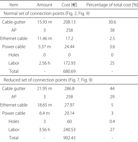
dot. Green cables represent power cables and red cables represent ethernet cables. The figures show that all APs are preferably located close to ECPs and PCPs, in order to reduce the amount of cables and cable gutters needed. Both configurations require 3 APs, but less cabling will have to be installed in Fig. 9a, due to the presence of more connection points, leading to a lower total cost. The right-most AP in Fig. 9b is relocated compared to Fig. 9a, in order to be located closer to an ECP.
Table 8 lists a cost analysis for the two connection point distributions. The individual costs are obtained from confidential interviews with wireless network deployment
Table 8Installation cost analysis for 54 Mbps
Item Amount Cost [e] Percentage of total cost [%]
Normal set of connection points (Fig. 2, Fig. 9)
Cable gutter 15.93 m 208.13 30.6
AP 3 258 38
Ethernet cable 11.46 m 17.2 2.5
Power cable 5.37 m 24.44 3.6
Holes 0 0 0
Labor 2.56 h 172.93 25
Total - 680.69
-Reduced set of connection points (Fig. 7, Fig. 9)
Cable gutter 21.95 m 286.8 44
AP 3 258 29
Ethernet cable 18.65 m 27.97 5
Power cable 6.4 m 29.14 3
Holes 3 60 0.4
Labor 3.56 h 240.53 27
-Fig. 10Resulting network layout for scenario III with indication of cabling (red dot/line= ethernet CP/cable,green dot/line= power CP/cable,purple dot= AP with EIRP indicated insidedot,colorsinside rooms (see legend) indicate ESL).aNormal set of connection points.bReduced set of connection points
companies. It shows that the configuration with fewer connection points indeed leads to a higher total cost: e902 vs.e681 or an increase of 32 %. Table 8 shows that this is due to the higher total cabling cost for connecting the rightmost AP in Fig. 9b to an ECP and to the higher labor cost associated with connecting this AP (drilling of three holes and installing more cables and cable gutters). The tables show that the AP cost is always below half of the total price, indicating the importance of performing a full cost analysis and not only accounting for the AP cost when planning wireless networks. Labor costs amount to about one-fourth of the total cost for both connection point configurations. The cost of the cables (6–8 %) is negligible compared to the cost of the cable gutters (31 and 44 % for the two configurations).
6.3 Scenario III: maximal coverage with minimal human exposure and minimal installation cost
Figure 10a and 10b shows the optimal layout of the network designed in scenario III for the configuration with a normal set and with a reduced set of connection points, respectively. The ESL distribution is indicated in the figures and is the same as the first distribution in scenario I. Again, optimal AP locations are close to the ECPs and PCPs, in order to reduce the cost. Addition-ally, they are also located in low-ESL rooms to keep the electric-field values low in high ESL rooms. Both configu-rations now require 4 APs, slightly more than when only
cost is accounted for (scenario II), but much fewer than when only exposure is accounted for (scenario I).
Table 9 compares the characteristics of the networks of scenario III with those of scenario I. Unlike in sce-nario I (exposure), scesce-nario III (cost+exposure) aims for a reduced installation cost. This cost indeed reduces from e4093 toe1086 (−73 %, normal CP set). The downside here is that field values are higher in scenario III:EESL50 and EESL95 increase from 57 to 62 mV/m (+9 %) and from 200 to 264 (+32 %), respectively, when changing from scenario I to III (normal CP set).
Table 9 also compares the characteristics of the net-works of scenario III with those of scenario II. Unlike in scenario II (cost), scenario III (cost + exposure) also aims for a reduced exposure.EESL50 andEESL95 decrease from 81 to 62 mV/m (–23 %) and from 417 to 264 mV/m (–37 %), respectively, when changing from scenario II to III for the configuration with the normal CP set. For the reduced
Table 9Overview of network characteristics for scenarios I-II-III
Scenario Installation cost [e] EESL
50 [mV/m] E95ESL[mV/m]
I: Normal CP set 4093 57 200
II: Normal CP set 681 81 417
II: Reduced CP set 902 84 373
III: Normal CP set 1086 62 264
III: Reduced CP set 1387 58 295
CP set, EESL50 and EESL95 decrease from 84 to 58 mV/m (–31 %) and from 373 to 295 mV/m (–21 %), respectively. The downside of the trade-off between installation cost and exposure is that in scenario III, the cost is higher than in scenario II:e1086 vs.e681 (+59 %) for the normal CP set, ande1387 vs.e902 (+54 %) for the reduced CP set. Reduced CP sets cause higher costs than normal CP sets (e902 vs.e681 for scenario II ande1387 vs.e1086 for scenario III) but have no influence on the field levels, as could be expected (see Table 9).
Scenario III (cost+exposure) is a good trade-off solu-tion between scenario I (exposure) and II (cost): the cost of scenario I is 601 % higher than that of the cost-optimized scenario II, while scenario III leads to a cost increase of only 59 % (normal CP set). Also, the EESL50 and E95ESL of scenario II are 49 and 208 % higher than in the exposure-optimized scenario I, respectively, while scenario III leads toEESL50 andEESL95 increases of only 9 and 32 %, respectively. Table 9 also lists the characteristics of the traditional sce-nario from [6] (scesce-nario REF), where coverage is provided with three 20 dBm APs, without accounting for exposure or full installation cost: only the number of APs is mini-mized. It shows that both exposure reduction (scenarios I and III) and cost reduction (scenarios II and III) are efficient in the proposed algorithm. As a summary, in sce-nario I, the lowest values ofEESL50 andEESL95 are obtained but this scenario results in the highest installation cost. On the contrary, scenario II has the lowest installation cost but corresponds to the highest exposure values. Scenario III provides trade-off solutions where both installation cost and exposure level are limited. Changing the weights of the fitness functions allows shifting between higher (lower) exposure and the corresponding lower (higher) installation costs.
6.4 Influence of interference margin (IM)
When WiFi networks are deployed, interference should be accounted for. The interference margin IM corresponds with an increase of the noise floor due to external inter-ference. Here, IM is assumed at 3 dB, but depending on the level of interference, different values can be assumed. Table 10 shows how interference influences the results for the three scenarios that are considered in this paper. For all scenarios, the coverage percentage for all situation remains 100 %. However, when accounting for interfer-ence, both the total installation cost and the exposure levels increase, since considering interference leads to higher EIRP levels or to a larger number of APs to main-tain the coverage rate. The installation cost,EESL50 , andE95ESL of scenario I increase frome4093 toe4114 (+0.5 %), from 57 to 68 mV/m (+16.2 %), and from 200 to 316 mV/m (+36.7 %), respectively, when changing including an IM of 3 dB. For scenario II, accounting for interference yields a solution with a cost ofe1152, which is 69 % higher than
Table 10Network characteristics for all scenarios, with and without considering an interference margin IM of 3 dB
Scenarios Coverage rate [%] Installation cost [e] EESL50 EESL95 rate [%] cost [e] [mV/m] [mV/m]
I without IM 100 4093 57 200
I with IM 100 4114 68 316
II without IM 100 680 85 417
II with IM 100 1152 93 529
III without IM 100 1081 61 263
III with IM 100 1453 80 353
before (e680). In scenario III, we obtain a cost ofe1453, anEESL
50of 80 mV/m, and anEESL95of 353 mV/m, com-pared toe1081, 61 mV/m, and 263 mV/m for scenario III without interference, respectively.
7 Conclusions
In this paper, an algorithm is presented for optimal indoor wireless network planning, based on a maximization of coverage and a minimization of the full installation cost (not only access point cost) and the human exposure. Advanced fitness functions are presented, accounting for the total installation cost in a realistic way, and introduc-ing exposure sensitivity levels per room. Three scenarios are defined and simulated. It is shown that a configura-tion with fewer possible connecconfigura-tion points for power and ethernet has a higher installation cost (+32 % for the con-sidered case). Further, the algorithm successfully reduces exposure levels in rooms that are defined as being sen-sitive to high electric-field values (average reductions of 50 % and more for the considered case). In a scenario where coverage, cost, and exposure are jointly optimized, a trade-off solution is found where the required coverage is provided, while keeping the total installation cost and the exposure levels limited. Accounting for interference leads to higher installation costs and higher exposure lev-els. Future research will consist of applying the proposed methods to heterogeneous networks, consisting of WiFi access points and LTE femtocells.
Competing interests
The authors declare that they have no competing interests.
Author details
1School of Computer Science and Engineering, University Electronic Science
and Technology of China, No.2006, Xiyuan Ave, 611731 Chengdu, China.
2Ghent University/iMinds, Dept. of Information Technology, Gaston
Crommenlaan 8 box 201, 9050 Gent, Belgium.
Received: 4 September 2014 Accepted: 10 July 2015
References
2. E Amaldi, A Capone, M Cesana, F Malucelli, F Palazzo, inVehicular Technology Conference, 2004. VTC 2004-Spring. 2004 IEEE 59th. WLAN coverage planning: optimization models and algorithms, vol. 4, (2004), pp. 2219–2223. doi:10.1109/VETECS.2004.1390668
3. M Deruyck, E Vanhauwaert, D Pareit, B Lannoo, W Joseph, L Martens, WiMAX based monitoring network for a utility company: a case study. Transactions on Emerging Telecommunications Technologies (2012). accepted doi:10.1002/ett.2573
4. G Koutitas, T Samaras, Exposure minimization in indoor wireless networks. Antennas Wireless Propagation Lett. IEEE.
9, 199–202 (2010)
5. D Plets, W Joseph, K Vanhecke, L Martens, inAntennas and Propagation Society International Symposium (APSURSI), 2012 IEEE. A heuristic tool for exposure reduction in indoor wireless networks (Chicago, IL, 2012), pp. 1–2
6. D Plets, W Joseph, K Vanhecke, L Martens, Exposure optimization in indoor wireless networks by heuristic network planning. Prog. Electromagnetics Research-Pier.139, 445–478 (2013)
7. K Jaffres-Runser, J-M Gorce, S Ubeda, inVehicular Technology Conference, 2006. VTC-2006 Fall. 2006 IEEE 64th. Multiobjective QoS-oriented planning for indoor wireless LANs (Montreal, Que, 2006), pp. 1–5
8. L Nagy, inAntennas and Propagation, 2007. EuCAP 2007. The Second European Conference On. Indoor radio coverage optimization for WLAN (Edinburgh, 2007), pp. 1–6
9. Z Yun, S Lim, MF Iskander, An integrated method of ray tracing and genetic algorithm for optimizing coverage in indoor wireless networks. Antennas Wireless Propagation Lett. IEEE.7, 145–148 (2008)
10. N Liu, D Plets, SK Goudos, W Joseph, L Martens, Multi-objective network planning optimization algorithm: human exposure, power consumption, cost, and coverage. Wireless Netw.21(3), 841–857 (2015)
11. D Plets, N Machtelinckx, K Vanhecke, JV Ooteghem, K Casier, M Pickavet, W Joseph, L Martens, inIEEE International Symposium on Antennas and Propagation and USNC-URSI Radio Science Meeting. Calculation tool for optimal wireless design and minimal installation cost of indoor wireless LANs (Memphis, TN, 2014)
12. JMB OLiveira, S Silva, LM Pessoa, D Coelho, HM Salgado, JCS Castro, in Microwave Photonics (MWP), 2010 IEEE Topical Meeting On. UWB radio over perfluorinated GI-POF for low-cost in-building networks (Montreal, QC, 2010), pp. 317–320
13. A Das, A Nkansah, NJ Gomes, IJ Garcia, JC Batchelor, D Wake, Design of low-cost multimode fiber-fed indoor wireless networks. Microwave Theory Tech. IEEE Trans.54(8), 3426–3432 (2006)
14. R Patra, S Surana, S Nedevschi, E Brewer, inProceedings of the Second ACM SIGCOMM Workshop on Networked Systems for Developing Regions. NSDR ’08. Optimal scheduling and power control for TDMA based point to multipoint wireless networks (ACM New York, NY, USA, 2008), pp. 7–12
15. M Yigitel, O Incel, C Ersoy, Dynamic base station planning with power adaptation for green wireless cellular networks. EURASIP J. Wireless Commun. Netw.2014(1), 77 (2014)
16. L Suarez, L Nuaymi, J-M Bonnin, An overview and classification of research approaches in green wireless networks. EURASIP J. Wireless Commun. Netw.2012(1), 142 (2012)
17. Y Lee, K Kim, Y Choi, inLocal Computer Networks, 2002. Proceedings. LCN 2002. 27th Annual IEEE Conference On. Optimization of AP placement and channel assignment in wireless LANs (Washington, DC, USA, 2002), pp. 831–836
18. C-K Ting, C-N Lee, H-C Chang, J-S Wu, Wireless heterogeneous transmitter placement using multiobjective variable-length genetic algorithm. Syst. Man Cybernet. Part B: Cybernetics, IEEE Tran.39(4), 945–958 (2009) 19. L Arya, SC Sharma, inProceedings of the Second International Conference on
Soft Computing for Problem Solving (SocProS 2012), December 28-30, 2012. Advances in Intelligent Systems and Computing, ed. by BV Babu, A Nagar, K Deep, M Pant, JC Bansal, K Ray, and U Gupta. Coverage of indoor WLAN in obstructed environment using particle swarm optimization, vol. 236, (2014), pp. 1583–1594. doi:10.1007/978-81-322-1602-5_157
20. G Mateus, AF Loureiro, R Rodrigues, Optimal network design for wireless local area network. Ann. Oper. Res.106(1–4), 331–345 (2001)
21. SW Ellingson, inVehicular Technology Conference, 2005. VTC-2005-Fall. 2005 IEEE 62nd. Antenna design and site planning considerations for MIMO, vol. 3, (2005), pp. 1718–1722
22. T Kikuchi, D Sugita, inIntelligent Green Building and Smart Grid (IGBSG), 2014 International Conference On. A method of an efficient installation process for generic cabling inside customer premises (Taipei, 2014), pp. 1–4 23. P Valberg, T van Deventer, M Repacholi, Workgroup report: base stations
and wireless networks–radio frequency (RF) exposures and health consequences. Environ Health Perspect.115(3), 416–424 (2007) 24. W Joseph, L Verloock, F Goeminne, G Vermeeren, L Martens, Assessment
of general public exposure to LTE and RF sources present in an urban environment. Bioelectromagnetics.31, 576–579 (2010)
25. L Verloock, W Joseph, G Vermeeren, L Martens, Procedure for assessment of general public exposure from WLAN in offices and in wireless sensor network testbed. Health Phys.98, 628–638 (2010)
26. W Joseph, P Frei, M Roosli, G Thuroczy, P Gajsek, T Trcek, J Bolte, G Vermeeren, E Mohler, P Juhasz, V Finta, L Martens, Comparison of personal radio frequency electromagnetic field exposure in different urban areas across Europe. Environ. Res.110, 658–663 (2010) 27. CGP Russo, V Vespasiani, A numerical coefficient for evaluation of the
environmental impact of electromagnetic fields radiated by base stations for mobile communications. Bioelectromagnetics.31(8), 613–621 (2010) 28. H Chen, Y Zhu, K Hu, T Ku, RFID network planning using a multi-swarm
optimizer. J. Netw. Comput. Appl.34(3), 888–901 (2011). RFID Technology, Systems, and Applications
29. D Jourdan, OL de Weck, inVehicular Technology Conference, 2004. VTC 2004-Spring. 2004 IEEE 59th. Layout optimization for a wireless sensor network using a multi-objective genetic algorithm, vol. 5, (2004), pp. 2466–24705. doi:10.1109/VETECS.2004.1391366
30. G Cerri, R De Leo, D Micheli, P Russo, Base-station network planning including environmental impact control. Commun. IEEE Proc.151(3), 197–203 (2004)
31. M Deruyck, W Joseph, B Lannoo, D Colle, L Martens, Designing energy-efficient wireless access networks: LTE and LTE-Advanced. Internet Comput. IEEE.17(5), 39–45 (2013)
32. I Vilovic, N Burum, Z Sipus, R Nad, inApplied Electromagnetics and Communications, 2007. ICECom 2007. 19th International Conference On. PSO and ACO algorithms applied to location optimization of the wlan base station (Dubrovnik, 2007), pp. 1–5
33. L Nagy, Global optimization of indoor radio coverage. AUTOMATIKA: ˇcasopis za automatiku, mjerenje, elektroniku, raˇcunarstvo i komunikacije. 53(1), 69–79 (2012)
34. S-Y Yang, D-W Seo, N-H Myung, in2010 International Symposium on Antennas and Propagation. Optimal location and number of access points based on ray-tracing and particle swarm optimization (Macau, China, 2010)
35. A Eisenblatter, H-F Geerdes, I Siomina, inWorld of Wireless, Mobile and Multimedia Networks, 2007. WoWMoM 2007. IEEE International Symposium on A. Integrated access point placement and channel assignment for wireless lans in an indoor office environment (IEEE Espoo, Finland, 2007), pp. 1–10
36. J Zhang, X Jia, Z Zheng, Y Zhou, Minimizing cost of placement of multi-radio and multi-power-level access points with rate adaptation in indoor environment. Wireless Commun. IEEE Trans.10(7), 2186–2195 (2011) 37. AW Reza, MS Sarker, K Dimyati, A novel integrated mathematical
approach of ray-tracing and genetic algorithm for optimizing indoor wireless coverage. Progress Electromagnetics Res.110, 147–162 (2010) 38. D Plets, W Joseph, K Vanhecke, E Tanghe, L Martens, Coverage prediction
and optimization algorithms for indoor environments. EURASIP J. Wireless Commun. Netw.2012, 123 (2012)