On the estimates of the ring current injection and decay
P. Ballatore1and W. D. Gonzalez2
1Istituto di Scienza e Tecnologie dell’Informazione, National Research Council, Via Moruzzi, 1-56124 Pisa, Italy 2National Institute for Space Research (INPE), S´ao Jos´e dos Campos, Brazil
(Received February 13, 2003; Revised June 23, 2003; Accepted August 7, 2003)
In the context of the space weather predictions, forecasting ring current strength (and of theDstindex) based on the solar wind upstream conditions is of specific interest for predicting the occurrence of geomagnetic storms. In the present paper, we have studied separately its two components: the Dst injection and decay. In particular, we have verified the validity of the Burton’s equation for estimating the ring current energy balance using the equatorial electric merging field instead of the original parameter V Bs (V is the solar wind speed and Bs is the southward
component of the Interplanetary Magnetic Field, IMF). Then, based on this equation, we have used the phase-space method to determine the best-fit approximations for the ring current injection and decay as functions of the equatorial merging electric field (Em). Results indicate that the interplanetary injection is statistically higher than in
previous estimations usingV Bs. Specifically, weak but not-null ring current injection can be observed even during
northward IMF, when previous studies considered it to be always zero. Moreover, results about the ring current decay indicate that the rate of Dst decay is faster than its predictions derived by usingV Bs. In addition, smaller
quiet time ring current and solar wind pressure corrections are contributing toDstestimates obtained byEminstead
ofV Bs. These effects are compensated, so that the statisticalDstpredictions using the equatorial electric merging
field or usingV Bsare about equivalent.
Key words:Magnetospheric physics, ring current, modeling and forecasting.
1.
Introduction
Forecasting the geomagnetic activity and the occurrence of geomagnetic storms are considered as one of the main goals in recent space weather investigations. The most com-monly used index of geomagnetic storms is the Dst index. Therefore Dst forecasting has been widely attempted and accurateDst estimates can be presently computed based on interplanetary space observations (O’Brien and McPherron, 2000a).
TheDstindex is derived from the perturbations of the hor-izontal component of the geomagnetic field as measured by mid-latitude (or latitudes at about 20◦–30◦ from theCGM, Corrected GeoMagnetic, equator) ground stations and it is expressed in units nT. It represents the westward ring current formed around the Earth and associated with the occurrence of the geomagnetic storms (Mayaud, 1980; Gonzalezet al., 1994). In particular, the energy of the ring current is car-ried by energetic ions injected into the magnetosphere pow-ered by the mechanisms of reconnection between the inter-planetary magnetic field (IMF) and the magnetospheric field. Generally, reconnection occurs when the two fields have op-posite directions. At the sub-solar point, this occurs when theIMFis directed southward (in theGSMcoordinate sys-tem). Therefore the ring current energy input is considered proportional to the upstream parameterV Bs, whereV is the
solar wind speed and Bs is the southwardIMF Bz
compo-nent (Burtonet al., 1975). The original ring current energy
Copy right cThe Society of Geomagnetism and Earth, Planetary and Space Sciences (SGEPSS); The Seismological Society of Japan; The Volcanological Society of Japan; The Geodetic Society of Japan; The Japanese Society for Planetary Sciences.
balance equation is:
Dst/t =Q−Dst/τ (1)
whereτ is the Dst decay time constant and Q is the ring current energy injection expressed as a linear function of V Bs (Burtonet al., 1975). In Eq. (1), Dst represents the
Dst corrected by the effects of the solar wind pressure (or the associated magnetospheric currents) and the quiet time ring current
Dst=Dst−b.P1/2+c (2)
wherePis the solar wind pressure andbandcare constants. A review paper by O’Brien and McPherron (2000a) sum-marizes and compares previous results about Dst forecasts. The models presented in that paper are based on Eq. (1), which was originally reported by Burtonet al.(1975). Each model has different parametersQ,τ,bandcin Eqs. (1) and (2). Specifically, O’Brien and McPherron (2000b) consid-ered Q andτ as functions ofV Bs and derivedbandc(in
Eq. (2)) to be 7.26 nT/nPa1/2and 11 nT, respectively. TheQ function is different from zero (and in particular it is nega-tive) only forV Bs >0.49 mV/m, when it is:
Q[nT/h]= −4.4.(V Bs[mV/m]−0.49). (3)
The decay rate,τ, is a function ofV Bsand it is:
τ[h]=2.4.e9.74/(4.69+V Bs[mV/m]). (4)
Eqs. (3) and (4) give very good Dst forecasts according to Eqs. (1) and (2). Therefore these Q andτ are considered, respectively, as theeffectivering current interplanetary en-ergy injection and decay. However it might be questioned
1 .0
E (m V /m )
1 0 .0
0 .1
1 .0
1 0 .0
1 0 0 .0
-Q
(n
T
/h
)
-1 e x p (1 .8 1 lo g (E m )-0 .2 0 ) E > 0
0
E = 0
m
m
Q =
m
2 0 .0
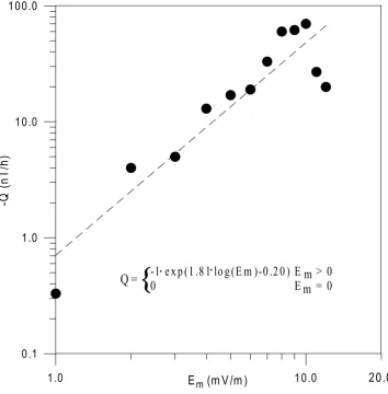
Fig. 1. InjectionQversusEm. Qvalues are derived from linear fits to the phase spaceDstvs.Dstfor separate 1 mV/mEmintervals; each point is shown at the center of theEminterval to which it refers.
how much theseeffective Qandτ differ from the real ones. In fact it is known that other quantities, besides theV Bs
pa-rameter, represent the interplanetary-magnetospheric recon-nection. For example, in this paper we consider the equato-rial projection of the merging electric field (Em), which
rep-resents the rectified reconnection electric field in the equato-rial plane (Gonzalez, 1990). Specifically, the equatoequato-rial Em
takes into account effects due to theIMF Bycomponent and
theIMFclock angle so that contributions from the reconnec-tions at the magnetospheric lobes are taken into account. In particular,Emcoincides withV Bsin the case of clock angle
close to 180◦orIMF ByBz with negativeBz.
The equatorial electric field considered here is (Kan and Lee, 1979; Akasofu, 1981):
Em=V Bt.sin2(φ/2) (5)
where Bt is the projection of theIMFon theY-Zplane (in
GSMcoordinate system) andφ is the clock angle between Btand theZ-axis (Kan and Lee, 1979).
This paper aims to look for the best approximations for the ring current injection and decay as functions ofEm.
Conclu-sions are based on the comparison between the present re-sults and previous findings ofQandτ usingV Bs instead of
Em.
2.
Data Analysis and Observations
The time interval under investigation is the period since January 1, 1995 until December 31, 2000. For this period, the interplanetary data considered are the measurements of IMFcomponents andV from the OMNI/NSSDC database. According to data availability, these measurements are from different satellites, mostly from WIND, but smaller amounts of the data are from IMP-8 and ACE. These measurements have been used to calculate theV BsandEmparameters.
A time delay is introduced between the ground basedDst index and the interplanetary data. This delay is chosen equal to 1-h in agreement with previous estimations of average delays between satellites and ground-based measurements (e.g., Ballatoreet al., 2001). It is worth mentioning that the 1-h delay is valid statistically, but not exactly at any specific time.
Using Eq. (1), we can calculate the offset and the slope of the linear best-fit for the scatter plots representingDstvs. Dstand we can deriveQandτ from the following equations
offset=Q.t (6)
slope= −t/τ (7)
0 .0 2 .0 4 .0 6 .0 8 .0 1 0 .0 1 2 .0
E (m V /m )
1 .0
1 0 .0
1 0 0 .0
(h
)
τ
= e x p (-0 .0 8 5 E + 2 .7 5 )
τ
m
m
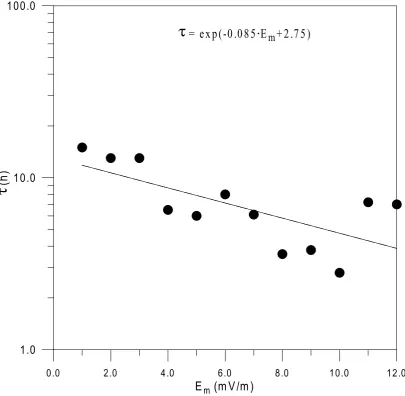
Fig. 2. DecayτversusEm.τvalues are derived from linear fits to the phase spaceDstvs.Dstfor separate 1 mV/mEmintervals; each point is shown at the center of theEminterval to which it refers.
the important dependence of Qandτ on the interplanetary parameters (e.g., Fenrich and Luhmann, 1998). However, if each scatter plot is limited only to data points with restricted intervals ofV Bs, the best-fits obtained are significant, andQ
andτ estimations (from Eq. (6) and Eq. (7)) can be consid-ered statistically significant too. Our procedure here is quite similar to that used by O’Brien and McPherron (2000b).
We have calculated the best-fits for the scatter plotsDst
vs. Dst considering data separated in 1 mV/m intervals of Em, starting from 0.05 mV/m until 12.5 mV/m. This is
simi-lar to the binning for separateV Bsintervals by O’Brien and
McPherron (2000b), but they calculated theDst vs. Dst best fits in eachV Bs sub-set, after having further averaged
these data in separateDstbins. In our case, the linear best-fit correlations take into account each data point measured and are significant at a confidence level above 99.9% untilEm∼
10.5 mV/m. However, the best correlations are found for the intervals withEm<8 mV/m, where most of the
interplane-tary data are observed. Above∼10.5 mV/m, the confidence level for the best fits are<99.0%, due to the small number of data points involved. TheQ andτ derived from Eq. (6) and Eq. (7) are shown in Figs. 1 and 2 as functions of the
correspondingEm(the data points are shown at the center of
the 1 mV/mEminterval to which they refer).
We have studied linear and non-linear fits in Figs. 1 and 2 between Qvs. Emandτ vs. Em, respectively. The
best-fits chosen forQ(Em)andτ(Em)(reported on the plots) are
the ones corresponding to the best correlation coefficients and the smallest residuals. The correlation coefficients for these two fits are 0.92 in Fig. 1 and 0.76 in Fig. 2 and cor-respond, respectively, to statistical confidence levels 99.9% and 99.2%. The possibility of defining quite significant best fits can be interpreted as the validity of Burton’s equation (Eq. (1)) by usingEminstead ofV Bs.
2.1 Ring current injectionQ
While the best fit betweenV Bsand Qis linear (O’Brien
and McPherron, 2000b), the best fit between Em and Q
is found to be a power law. This may suggest a strong relationship between the sub-solar point reconnection and the ring current energy input and a quite large magneto-spheric/ionospheric re-processing of the ring current energy injection originated by magnetospheric lobe reconnections.
-8 0 -6 0 -4 0 -2 0 0
Q (n T/h )
1 1 0 1 0 0 1 0 0 0 1 0 0 0 0
n
1 1 0 1 0 0 1 0 0 0 1 0 0 0 0
n
1 1 0 1 0 0 1 0 0 0 1 0 0 0 0
n
1 1 0 1 0 0 1 0 0 0 1 0 0 0 0
n
-1 6 0 -1 4 0 -1 2 0 -1 00 -8 0 -6 0 -4 0 -2 0 0
Q (n T/h )
|φ| > 160
110 < |φ| < 160
90 < |φ| < 110
IM F B > 0 nT
z
Q (E )
Q (V B ) m
s
Fig. 3. Number ofQoccurrences in the 5 nT/h intervals whose center is indicated on the abscissa. Each panel refers to periods when the clock angle was in the range indicated on the right. The bottom panel refers to periods ofIMF Bz>0.
V B2L2 sin4(φ/2), whereB is the module of the totalIMF vector andL is a scale length at the magnetopause) and the Dstindex. In this case, the best-fit was a second order poly-nomial function in log()f. This was explained by consider-ing that a more intense rconsider-ing current forms closer to the Earth, where the atmosphere density increases exponentially.
We have studied a quantitative comparison between the function Q(V Bs) calculated according to O’Brien and
McPherron (2000b) and theQ(Em)function given by:
log(−Q(Em))[nT/h]=1.81.log(Em[mV/m])−0.2. (8)
Results are shown in Fig. 3, where the number of oc-currences of Q(Em)and Q(V Bs)are reported for separate
ranges of theIMFclock angle during negativeIMF Bz(three
-0 .6 0
-0 .3 0
0 .0 0
0 .3 0
0 .6 0
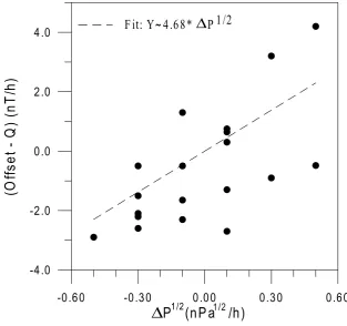
Fig. 4. Residual of phase space offsets minus the injectionQversus variations of the solar wind dynamic pressureP. The constantbin Eq. (2) is estimated by the slope of the fit and it is equal to 4.68.
nT/h Q interval to which it refers. It can be seen that the distribution ofQ(V Bs)is clustered at zero, with maximum
total occurrence (this total occurrence is the sum of the oc-currence in the three upper panels of Fig. 3) in the range between−5 nT/h and 0 nT/h. Differently, the distribution of Q(Em) is shifted towards higher injection values, with
maximum occurrence in the range between −10 nT/h and −5 nT/h for each one of the three upper panels in Fig. 3. The shift between Q(Em)and Q(V Bs)is especially clear
forIMFclock angle|φ| closer to 90◦, when the number of occurrences ofQ(Em)is always higher thanQ(V Bs)for
in-tervals ofQ<−5 nT/h.
The bottom panel of Fig. 3 shows the distribution of data points with Q(Em) different from zero for periods with
northwardIMF, when Q(V Bs)is always equal to zero.
Al-though, in this panel, most of the Q(Em)occurrences are
clustered towards zero, a significant percentage of data lies in the range (−25, 0) nT/h.
2.2 Ring current decayτ
The rate of the ring current decayτ calculated by O’Brien and McPherron (2000b) was based on the hypothesis that an increase in V Bs (i.e., during a higher magnetospheric
convection electric field) is associated with a shift towards lower altitudes of the boundary between open and closed drift orbits. At lower altitudes the denser exosphere pro-vides a more rapid charge exchange interactions, resulting in a more rapid decay of the ring current (O’Brien and McPher-ron, 2000b). In particular, it is assumed that τ is related to the charge exchange lifetime,τ ∝ (nH)−1, wherenH is
the density of hydrogen in the geocorona (Smith and Bew-tra, 1978). In addition, the geocorona density falls with
dis-tance from the Earth, L, as nH ∝ e−L/L0, where L0 is a scale height determined by atmospheric and gravitational pa-rameters (Smith and Bewtra, 1978). Therefore, O’Brien and McPherron (2000b) considered
τ ∝eL/L0 (9)
whereL is the distance from the Earth andL0is the scale height mentioned above. Considering0as the electric field strength proportional to the polar cap potential drop, results by Reiffet al.(1981) showed that
L−1∝0 (10)
Equation (12) (O’Brien and McPherron, 2000b) roughly in-dicates that a decrease inτ(V Bs)is associated with an
in-crease inV Bs. Similarly, in our case, we find that a decrease
inτ(Em)is associated with an increase inEm, with the best
functional form given by (see Fig. 2)
-3 0 -2 0 -1 0 0 1 0 2 0 3 0
D iffe re n ce s (n T )
0 3 0
n(
%
)
0 3 0
n(
%
)
0 3 0
n(
%
)
0 3 0
n(
%
)
0 3 0
n(
%
)
0 3 0
n(
%
)
0 3 0
n(
%
)
0 3 0
n(
%
)
D st-D st (V B )
D st-D st (E
m)
φ
φ φ
φ φ
φ φ φ φ
s
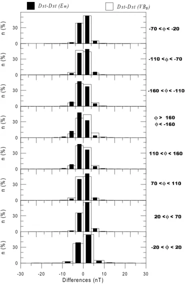
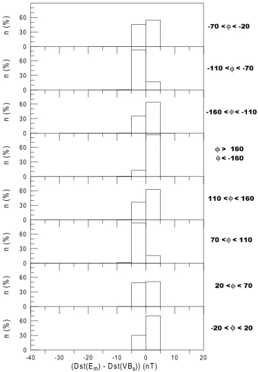
Fig. 5. Distributions of the differencesDst−Dst(Em)andDst−Dst(V Bs). Each panel refers to periods when the clock angle lies as indicated at the right of the plot.
2.3 Pressure correction and quiet time ring current The correction to Dst, introduced in Eq. (1) and related to the solar wind pressureP, takes into account the contribu-tion of the ring current energy balance due to magnetospheric currents (e.g., Burton et al., 1975; O’Brien and McPher-ron, 2000b). In order to estimate this pressure correction, we use a procedure quite similar to O’Brien and McPher-ron (2000b). For separate intervals of pressure variations,
the differences between the phase space best-fit offsets and Q(Em)(given by Eq. (8)) are calculated for separateEm
in-tervals. In each pressure variation range, this is done for each Eminterval in which there is a relatively sufficient number of
data points. In this case the definition of the offset given by Eq. (6) is extended to
-4 0 -3 0 -2 0 -1 0 0 1 0 2 0
Fig. 6. Distribution of the differencesDst(Em)−Dst(V Bs). Each panel refers to periods when the clock angle lies as indicated at the right of each plot.
More specifically, 1h data points for the whole period 1995– 2000 have been grouped for separate 0.2 nPa1/2/h intervals of variationP1/2. Then, separately for each of these groups, a procedure equal to that used for deriving Fig. 1 has been repeated to find the offsets for separate 1 mV/m intervals of Em. Finally, the differences between these offsets (in units
nT/h) and Q(Em)calculated from Eq. (8) have been found.
We show these differences in Fig. 4 as functions of the center of the corresponding 0.2 nPa1/2/h interval ofP1/2.
From Eq. (14) and the best-fit obtained in Fig. 4, we derive the coefficientb(that corresponds tobgiven in Eq. (2) and
Eq. (14)) as 4.68 nT/nPa1/2, which is smaller than the value 7.26 nT/nPa1/2derived usingV B
s(O’Brien and McPherron,
2000b). The best fit chosen has a correlation coefficient equal to about 0.64 with 19 data points, corresponding to a statistical confidence level equal to about 99.5%.
2000b) and it is also smaller than the original value of 20 nT, derived by Burtonet al.(1975).
The fact that the estimates of b andc obtained by Em
are smaller than those previously derived byV Bs indicates
smaller contributions from magnetopause currents due to the solar wind pressure and smaller level of the quiet time ring current. This might suggest that some of the power previously attributed to these processes is actually driven by IMF/magnetosphere reconnections occurring at magne-tospheric lobes, which are taken into account byEm.
2.4 Comparisons amongDstand its estimates as func-tions ofVBsandEm
TheDst forecast has been computed using interplanetary parameters according to Eq. (1) and the functions Q(V Bs)
and τ(V Bs) given by Eq. (3) and (4). In this way the
Dst(V Bs)is calculated as reported by O’Brien and
McPher-ron (2000a, b). Similarly, the Dst(Em)has been derived
by using Eq. (1) withQ(Em)andτ(Em)functions given in
Eq. (8) and (13), respectively.
As a further verification of the validity of Eq. (1) for the use ofEmand also to estimate the possible precision of the
Dst forecast obtained by Em, we compared the estimated
Dst(Em)and Dst(V Bs)with the observed Dst index. In
Fig. 5 the distributions of the differences Dst −Dst(Em)
andDst−Dst(V Bs)are reported for separate ranges of the
IMFclock angle. Both distributions maximize in the range (−5, 5) nT, where a percentage of data points>70% is ob-served. This indicates good precision of bothDst(V Bs)and
Dst(Em)predictions. In addition, the percentage of
occur-rences in the range (−5, 5) nT for Dst(Em) is about the
same as the distribution Dst(V Bs). Therefore, the
predic-tion of the ring current level made byEmcan be considered
as significant as that made byV Bs. In particular, in Fig. 5,
the distributions related toDst(Em)andDst(V Bs)are very
much similar for the clock angleφin the range(−70,70)◦, namely, during the most northwardIMFvalues.
We note that, in Fig. 5, the occurrences of differences in the positive range of the abscissa correspond to the occur-rences of aDst less disturbed than Dst(Em)or Dst(V Bs),
i.e.Dst(Em)orDst(V Bs)over-estimates the observedDst.
Similarly, the occurrence of differences in the negative range of the abscissa indicates that the corresponding Dst(Em)
or Dst(V Bs)under-estimates the measured Dst, which is
more disturbed. Therefore, Figure 5 shows that, for φ around 90◦, Dst(Em) tends to over-estimate the observed
Dst, while this is not so for Dst(V Bs). In fact, forφ in
the interval(70,110)◦and(−110,−70)◦, the occurrence of Dst−Dst(Em)is higher in the positive range, while the
oc-currence of Dst −Dst(V Bs)in the positive range is equal
to or smaller than in the negative range. These observations are in agreement with the occurrence of higher merging ob-served in Fig. 3 for clock angles closer to |90|◦. On the other hand, for the most southward orientedIMFvalues (φ around 180◦),Dst(Em)tends to under-estimate theDst
in-dex, whileDst(V Bs)tends to over-estimate it.
Figure 5 shows that the observed results are rather sym-metrical for positive or negative clock angle ranges, so that no significant differences are presently obtained for positive or negativeIMF Byperiods.
A more direct comparison between Dst(Em) and
Dst(V Bs)is given in Fig. 6, where the distributions of the
differences Dst(Em)−Dst(V Bs)are reported for separate
ranges of theIMFclock angle. It is shown that Dst(V Bs)
tends to indicate a ring current activity higher thanDst(Em)
does, except at clock angles around 90◦(φ=(−110,−70)◦ and φ = (70,110)◦), when Dst(Em) is more disturbed.
The higher ring current level estimated by Dst(V Bs)than
Dst(Em)is not due to the higher injectionQ(V Bs), which
is zero during northwardIMFand tends to be smaller than Q(Em)also during the other periods (as indicated in Fig. 3).
Therefore this higher disturbance indicated by Dst(V Bs)
compared with Dst(Em)can be in part attributed to larger
contributions to Dst(V Bs) from the quiet time Dst and
from the solar wind pressure correction (Section 2.3) and in part to the fact that τ(V Bs)is higher than τ(Em)
(Sec-tion 2.2). In particular, these factors seems to compensate the absence of injection for Dst(V Bs)during northwardIMF.
However, the estimates of the ring current injection and de-cay byEmare better than that byV Bs. In fact,Emconsiders
interplanetary-magnetospheric merging as indicated byV Bs
and additional magnetospheric-lobe effects (Akasofu, 1981; Gonzalez, 1990).
3.
Conclusions
The present study of the ring current energy balance demonstrates the validity of using Em in predicting Dst
(Eq. (1)) (Burtonet al., 1975) instead of the parameterV Bs.
In fact, the Dst predictions obtained using Em agree well
with the observedDst. We have given new functional forms for the ring current injection (Q) and decay (τ) in term of Em.
The estimate of Q as a function ofEm indicates the
oc-currence of an interplanetary injection greater than that cal-culated using V Bs. This effect is particularly evident for
IMFclock angles|φ|closer to 90◦, when the reconnection between the magnetosphere and the interplanetary magnetic field is more active on the magnetospheric lobes. In addi-tion, during positiveIMF Bzperiods, whenQcalculated
us-ing V Bs is always zero (Burtonet al., 1975; O’Brien and
McPherron, 2000a, b), the injection estimated using Em is
generally in the range (0, 25) nT.
The prediction of the rate of ring current decay, τ, ob-tained by usingEmindicates that the real loss should be more
rapid than that calculated in previous forecasts. In addition, a smaller level of quiet time ring current and a smaller solar wind pressure correction are obtained using Em instead of
V Bs.
The comparison between Dst predictions produced by V Bs or by Em shows comparable accuracy. Therefore, we
do not promote using Em instead of V Bs, but we merely
highlight thatEmcould be alternatively used instead ofV Bs
inDstforecasts.
Acknowledgments. The interplanetary data and the geomagnetic indexDstare from the OMNI database, U.S. National Space Sci-ence Data Center (NASA, Goddard Space Flight Center, USA).
References
magneto-sphere,Space Sci. Rev.,28, 121–190, 1981.
Ballatore, P., J. P. Villain, N. Vilmer, and M. Pick, The influence of inter-planetary medium on SuperDARN scattering occurrence,Ann. Geophys-icae,18, 1576–1583, 2001.
Burton, R. K., R. L. McPherron, and C. T. Russell, An empirical relationship between interplanetary conditions and Dst,J. Geophys. Res.,80, 4204– 4214, 1975.
Fenrich, F. R. and J. G. Luhmann, Geomagnetic response to magnetic clouds of different polarity,Geophys. Res. Lett.,25, 2999–3002, 1998. Gonzalez, W. D., A unified view of solar wind—magnetosphere coupling
functions,Planet. Space Sci.,38, 627–632, 1990.
Gonzalez, W. D., J. A. Joselyn, Y. Kamide, H. W. Kroehl, G. Rostoker, B. T. Tsurutani, and V. M. Vasyliunas, What is a geomagnetic storm?,J. Geophys. Res.,99, 5771–5792, 1994.
Kan, J. R. and L. C. Lee, Energy coupling function and solar wind— magnetosphere dynamo,Geophys. Res. Lett.,6, 577–580, 1979.
Mayaud, P. N.,Derivation, Meaning and Use of Geomagnetic Indices, Geo-phys. Monograph, vol. 22, AGU, Washington, DC, 1980.
O’Brien, T. P. and R. L. McPherron, Forecasting the ring current index Dst in real time,J.A.S.T.P.,62, 1295–1299, 2000a.
O’Brien, T. P. and R. L. McPherron, An empirical phase space analysis of ring current dynamics: Solar wind control of injection and decay,J. Geophys. Res.,105, 7707–7720, 2000b.
Reiff, P. H., R. W. Spiro, and T. W. Hill, Dependence of polar cap potential drop on interplanetary parameters, J. Geophys. Res.,86, 7639–7648, 1981.
Smith, P. H. and N. K. Bewtra, Charge exchange lifetime for ring current ions,Space Sci. Rev.,22, 301–318, 1978.