Nonlinear Image Restoration Using a Radial Basis
Function Network
Keiji Icho
The Research & Development Department, Matsushita Electric Industrial Co., Ltd., Osaka 571-8501, Japan Email:[email protected]
Youji Iiguni
Department of Systems Innovation, Graduate School of Engineering Science, Osaka University, Osaka 560-8531, Japan Email:[email protected]
Hajime Maeda
Department of Communications Engineering, Graduale School of Engineering, Osaka University, Osaka 565-0871, Japan Email:[email protected]
Received 4 August 2003; Revised 22 April 2004
We propose a nonlinear image restoration method that uses the generalized radial basis function network (GRBFN) and a regu-larization method. The GRBFN is used to estimate the nonlinear blurring function. The reguregu-larization method is used to recover the original image from the nonlinearly degraded image. We alternately use the two estimation methods to restore the original image from the degraded image. Since the GRBFN approximates the nonlinear blurring function itself, the existence of the in-verse of the blurring process does not need to be assured. A method of adjusting the regularization parameter according to image characteristics is also presented for improving restoration performance.
Keywords and phrases:radial basis function network, regularization, nonlinear image restoration, steepest descent technique, alternate estimation.
1. INTRODUCTION
In the recent years, a special class of artificial neural net-works, called the radial basis function network (RBFN), has received considerable attention [1]. The RBFN has a univer-sal approximation capability [2] and has successfully been applied to many signal and image processing problems due to its excellent approximation capability [3,4]. The RBFN provides a smooth function that achieves a good tradeoff be-tween fidelity to the data and smoothness. The regularization parameter controls the tradeoff between the two require-ments. In the standard RBFN, the number of basis functions is set to equal to the number of data. Therefore, the com-putational requirement of constructing the RBFN gets larger as the number of data gets larger. For reducing the compu-tational complexity, the generalized RBFN (GRBFN), which has a smaller number of basis functions than the number of data, has been proposed [1,5].
Restoration of images degraded by blur and additive noise is very important in image processing. A number of image restoration methods have been proposed so far
[6,7,8,9]. In [8], a regularization approach has been de-veloped, which provides a compromise between fidelity of the restored image to the degraded image and smoothness of the original image and the blurring function. Alternate estimation of original image and blurring function is em-ployed for improving restoration performance, however the blurring function is assumed to be linear. In some applica-tions, nonlinear blurring needs to be considered in the de-sign of restoration process. The neglect results in an unac-ceptable restoration performance [10]. In [9], the GRBFN is used to restore the original image from the nonlinearly de-graded image in the presence of observation noise, however the inverse of the blurring process is assumed to exist. More-over, the GRBFN trained by a training image has been fixed during the processing of test images.
under the assumption that the blurring function is known and smooth. A cost function is then minimized by using the steepest descent technique. In actual applications, nei-ther the blurring function nor the original image is known. We thus alternately use the two estimation methods to re-store the original image from the nonlinearly degraded im-age, under the single assumption of the smoothness of orig-inal image and blurring function. Since the GRBFN ap-proximates the nonlinear blurring function itself, the exis-tence of the inverse of the blurring process does not need to be assured. Moreover, in order to efficiently remove noise components, we propose a method of adjusting the regu-larization parameter according to image characteristics. It is shown through computer simulations that the adaptive selection method is useful in improving restoration perfor-mance.
2. FUNCTION APPROXIMATION
BY USING THE GRBFN
2.1. RBFN
Suppose that the I/O relationship between thep-dimensional input vectorx=[x1,x2,. . .,xp]T and the scalar output yis described by
y=g(x) +ε, (1)
where g is an unknown function, andεis a random noise with zero mean. Given a set ofNobservations{(xi,yi)}Ni=1, the regularization procedure determines a smooth function
f that minimizes the following cost function:
H[g]= N
i=1
yi−g
xi2+λS[g]. (2)
The first term measures the distance between the data and the desired solution. The second term is the stabilizer that mea-sures the cost associated with the deviation from the smooth-ness. The nonnegative parameterλ, called the regularization parameter, controls the tradeoffbetween the two terms. Asλ
is larger, the resulting function becomes smoother, while the discrepancy between the data point and the network output becomes larger.
We choose the stabilizer as
S[g]=
∞
n=0
(−1)nσ2n
n!2n∇
2ng, (3)
where∇2nis theniterated Laplacian operator inn dimen-sions. Then, the minimization ofH[g] yields the following solution [1]:
g(x)= N
i=1
cihx−xi, (4)
whereciandxiare the network parameter and the RBF cen-ter, respectively, andhis the Gaussian function defined by
hx−xi=exp
−x−xi 2
2σ2
. (5)
The parameterσ is the width of the Gaussian function. The function g is called the RBFN as it is expressed as a linear combination of RBFs,h(|x−xi|) (i=1, 2,. . .,N). The net-work parameter is determined by solving the following linear equations of size (N×N):
(H+λI)c=y. (6)
Here, y = [y1,y2,. . .,yN]T is the output vector,c = [c1,
c2,. . .,cN]T is the parameter vector, and His the (N×N) matrix whosei jth element is given by (H)i j =h(|xi−xj|). The matrix (H+λI) is always invertible for nonnegativeλ
[11]. The RBFN has a universal approximation capability [2] and has successfully been used for approximating a large va-riety of nonlinear functions in signal and image processing problems [3,4].
2.2. GRBFN
The GRBFN, which has a smaller number of basis functions than the number of data, is represented by [1,5]
g(x)= M
j=1
cjexp
−x−tj 2
2σ2
, (M < N), (7)
where M is the number of basis functions and the p -dimensional vectortj (j = 1, 2,. . .,M) is called the center of the GRBF. The network parametercj(j =1, 2,. . .,M) is determined by solving the following linear equations of size (M×M),
GTG+λG 0
c=GTy, (8)
where we define the (N×M) matrixGand the (M×M) matrixG0as
(G)i j=exp
−xi−tj 2
2σ2
(i=1, 2,. . .,N, j=1, 2,. . .,M),
G0
pq =exp
−tp−tq 2
2σ2
(p,q=1, 2,. . .,M),
(9)
respectively, and put c = (c1,c2,. . .,cM)T and y = (y1,
y2,. . .,yN)T. We putM = N to haveG = G0 = H. The GRBFN then results in the standard RBFN.
N
N
X1 X2
XN+1 XN+2
XN
X2N
XN2
. . . · · · · · ·
···
Figure1: Pixel positionxi.
Degraded image Blurred
image Original
image
yi
g(fi)
f(xi)
g
εi
+
Figure2: Degradation process.
xi−N−1 xi−N xi−N+1 xi−1 xi xi+1 xi+N−1 xi+N xi+N+1
Figure3: Pixel position considered infi.
3. IMAGE RESTORATION BASED ON THE REGULARIZATION METHOD
We express the original image of size (N×N) as f(xi) (i= 1, 2,. . .,N2), where we choose the pixel positionxias shown inFigure 1.Figure 2illustrates the degradation process con-sidered here. The degraded imageyiat the positionxiis rep-resented by
yi=g
fi+εi
i=1, 2,. . .,N2, (10)
wheregis a space-invariant nonlinear blurring function,εiis a random observation noise with zero mean. Also,fiis the 9-dimensional vector (or the (3×3) image) consisting of pixel values of the original image atxiand its 8-nearest neighbors, represented by
fi=fxi−N−1
,fxi−N
,fxi−N+1
,fxi−1
,
fxi,fxi+1,fxi+N−1
,fxi+N,fxi+N+1T. (11)
Figure 3illustrates the pixel position of the elements offi. Al-though we here definefias in (11), other choices are possible. We estimate the blurring functiong from the degraded image yi by using the GRBFN, under the assumption that the original image f(xi) is known andgis smooth. Next, we
N
N M N M N M N M
N M
N M
N M
N M N
· · ·
· · ·
· · ·
· · · .
. . . . . . .
. ···
Figure4: Pixel positions of the centers.
estimate f(xi) fromyiby using a regularization method, un-der the assumption thatgis known and f(xi) is smooth. Fi-nally, we alternately use the two methods to estimate f(xi) fromyi, under the single assumption of the smoothness ofg and f(xi).
3.1. Estimation of blurring function
We approximate the smooth blurring functiong(fi) by using the GRBFN with M2 centers. The output of the GRBFN is represented by
gfi=
M2
j=1
cjexp
−fi−tj 2
2σ2
, (12)
where g denotes the estimate of g. We here put the 9-dimensional centertjas
tk+M(l−1)=f(N2/M)(l−1)+(N/M)(k−1)+N+2 (k,l=1, 2,. . .,M),
(13)
so that they are equally distributed over the whole image space. The black squares inFigure 4denote the positions of the center. For example, when N = 256 andM = 4, the GRBFN has 16 centers such thatt1=f258,t2=f322,. . .,t16= f49602.
Table1: MSE for different values ofλandσ2, (E[ε2
i]=200).
σ2 λ
0.0001 0.001 0.01 0.1 1.0 100 180.96 180.96 180.96 180.96 180.96 200 14.10 14.10 14.10 14.10 14.11 500 2.45 2.45 2.45 2.47 2.74 1000 2.31 2.30 2.33 2.61 3.08 2000 2.57 2.58 2.76 2.81 2.88 10000 2.82 2.82 2.80 3.02 16.97
The regularization parameterci(i =1, 2,. . .,M2) is de-termined by solving the following linear equations of size (M2×M2):
GTG+λG0c=GTy, (14)
where we define the (N2×M2) matrixGand the (M2×M2) matrixG0as
(G)i j
=exp
−fi−tj
2
2σ2
, i=1, 2,. . .,N2, j=1, 2,. . .,M2,
G0
pq=exp
−tp−tq 2
2σ2
, p,q=1, 2,. . .,M2,
(15)
respectively, and put c = (c1,c2,. . .,cM2)T and y = (y1, y2,. . .,yN2)T. Although we may no longer find physical
prop-erties of the blurring process from (12), the GRBFN can ap-proximate an arbitrary nonlinear function with high accu-racy [11].
3.2. Example of blur estimation
We here consider the following nonlinear blurring function:
gfi=1 3
f2xi
−N−1
+f2xi
−N
+f2xi
−N+1
+ f2xi
−1
+f2xi+f2xi+1
+ f2xi+N−1
+ f2xi+N+ f2xi+N+11/2.
(16)
We degraded the Girl image of size (256×256) with 8 bit grayscale by using (16). Using the degraded image, we mea-sured the computation time and the mean square error (MSE) between the true and approximated images, com-puted by
MSE= 1
N2 N2
i=1
gfi−gfi2. (17)
As the number of basis functionsMincreases, the MSE be-comes smaller, while the computation time bebe-comes larger. Therefore, we have to make a tradeoffbetween the computa-tion time and the MSE in determining the parameterM.
Table2: MSE for different values ofλandσ2, (E[ε2
i]=400).
σ2 λ
0.0001 0.001 0.01 0.1 1.0 100 180.99 180.99 180.99 180.99 180.98 200 14.15 14.15 14.15 14.15 14.16 500 2.51 2.51 2.51 2.52 2.76 1000 2.36 2.36 2.38 2.64 3.10 2000 2.62 2.63 2.81 2.84 2.89 10000 2.84 2.84 2.82 3.03 16.92
We measured the computation time for different values ofM, where we used an IBM PC/AT compatible computer with an Intel Pentium II 750 MHz and 256 MB DRAM. The computation times for M = 2, 4, 8, 16 are 0.95, 6.15, 78.4, and 1226.6 (s), respectively. We next measured the MSE for different values ofλandσ2, where we putM = 4. Tables1 and2summarize the results forE[ε2
i] = 200 andE[ε2i] = 400, respectively. We see that choosingλ =0.001 andσ2 = 1000 provides a good tradeoffbetween the computation time and the MSE, and that the MSE is fairly robust against the choice. From these results, we put M = 4,λ = 0.001, and
σ2=1000 throughout the simulations.
3.3. Estimation of original image
We assume that the blurring functiong is known and use a regularization method to estimate f(xi) fromyi. We choose a cost function to be minimized as
J[F]= N2
i=1
yi−g
fi2
+γ
N2
i=1
fxi−N
+ fxi−1
−4fxi
+ fxi+1+ fxi+N 2,
(18)
where F def= [f(x1),f(x2),. . .,f(xN2)]T denotes the vector
representation of the original image. The first term measures the distance between the degraded and blurred images, and the second term is the Laplacian operator that measures the smoothness of the original image. The regularization param-eterγcontrols the tradeoffbetween the two terms. We here use the following steepest descent method for the minimiza-tion:
fk+1xi=fkxi− µ
N2
∂J ∂ fxi
F=Fk
i=1, 2,. . .,N2,
(19)
where µ is a small positive constant called the step size, and Fk = [fk(x1),fk(x2),. . .,fk(xN2)]T denotes the
3.4. Alternate estimation of blurring function and original image
In the blur estimation described inSection 3.1, the original image f(xi) is assumed to be known. In the original image estimation described inSection 3.3, the blur functiong(fi) is assumed to be known. However, in actual applications, nei-ther the original image nor the blurring function is known. Therefore, we alternately use the blur and image estimation methods.
We prepare a clean original image, and generate a train-ing image by blurrtrain-ing the original image and addtrain-ing observa-tion noise to the blurred image. We apply the blur estimaobserva-tion method to the training image under the assumption that the original image is known. We denote the initial estimate of the blurring function byg. The training image is used only for obtaining g. We call the degraded image to be restored the test image. Unlike the training image, we assume that the original image of the test image is unknown. We replace the blurring functiongin (18) by the initial estimategto have
J[F]= N2
i=1
yi−g
fi2
+γ
N2
i=1
fxi−N
+fxi−1
−4fxi
+fxi+1+fxi+N 2.
(20)
We minimize the cost function (20) with respect toFby us-ing the steepest descent method (19), and obtain the restored imageFk. In general, the initial estimategis not accurate. We thus replace f(xi) byfk(xi) in (14) and (15), and again esti-mate the blurring function by solving the linear equations (14). We alternately repeat the estimations of the blurring function and the original image until the iteration (19) con-verges. The blur function is uniquely estimated by solving (14), while the original image is iteratively estimated by us-ing the steepest descent method (19) so that the cost function
J[F] is minimized. SinceJ[F] is nonlinear with respect toF, the steepest descent method may converge to local minima ofJ.
4. SIMULATION RESULTS
Using Girl, Lena, and Baboon images of size 256×256 with 8-bit gray levels, we evaluated the restoration performance of the proposed method. We generated the training image by using the following blurring function:
gfi=1 3
f2xi
−N−1
+ 1.1f2xi
−N
+ 0.9f2xi
−N+1
+ 0.8f2xi
−1
+f2xi+ 1.2f2xi+1
+ 0.9f2xi+N
−1
+ 1.1f2xi+N+ f2xi+N+1 1/2, (21)
while we generated the test images by using (16). It is here noted that the blurring functions are different in the training
(a) (b)
(c) (d)
Figure 5: Blur estimation result: (a) original image f(xi), (b)
blurred imageg(fi), (c) degraded imageyi, and (d) output of the
GRBFNg(fi).
and test images. Throughout the simulations, we putE[ε2i]= 200.
We used the degraded Girl image as the training image, the degraded Lena and Baboon images as the test images, and compared the restoration performances of the following two methods.
Method A
This method comprises two steps.
Step (1) Using the training image, we initially estimate the blurring function by the GRBFN.
Step (2) Using the test image, we repeat the update proce-dure (19) to estimate the original image until no significant improvement is obtained.
Method B
This method comprises four steps.
Step (1) Using the training image, we initially estimate the blurring function by the GRBFN.
Step (2) Using the test image, we repeat the update proce-dure (19) 10 times to obtain a restored image at an intermediate stage.
Step (3) We regard the restored image as the original im-age, and again estimate the blurring function. Step (4) Repeat Step (2) and Step (3) until no significant
improvement is obtained in Step (2).
140 120 100 80 60 40 20 0
Number of iterations 0
0.5 1 1.5 2
SNRI
(dB)
A B
(a)
140 120 100 80 60 40 20 0
Number of iterations 0
0.5 1 1.5 2
SNRI
(dB)
A B
(b)
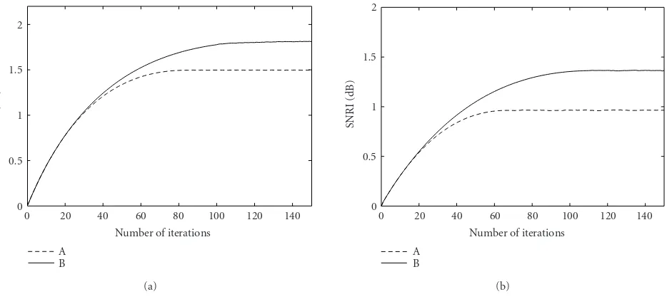
Figure6: Convergence curves of SNRIs made by Methods A and B: (a) Lena and (b) Baboon.
test images, while in Method B, both of the blurring function and the original image are iteratively estimated. We can verify the usefulness of the alternate estimation by comparing the restoration performance of Methods A and B.
Figure 5shows the blur estimation result obtained by us-ing the trainus-ing image. Figures5a,5b, and5cshow the orig-inal, blurred, and degraded Girl images, respectively, and Figure 5dshows the output of the GRBFN. We see thatg(fi) and g(fi) are very close to each other. We measured the signal-to-noise ratio improvement (SNRI) for each iteration, defined by
SNRI=SNR offkxi−SNR ofy i
=10 log10
N2
i=1 f2
xi
N2
i=1fk
xi−fxi2
−10 log10
N2
i=1f2
xi
N2
i=1
yi−f
xi2
=10 log10
N2
i=1
yi−f
xi2
N2
i=1fk
xi−fxi2.
(22)
Figure 6shows the convergence behaviors of SNRI for Meth-ods A and B, where Figures6aand6bare the results of Lena and Baboon images, respectively. The horizontal axis denotes the total number of iterations in the steepest descent method. We putµ=0.02 so that the SNRI is higher and the recursion (19) converges in 100 iterations. This means that the number of turns from Step (4) to Step (2) is 9=100/10−1. We see that Method B gives a better restoration performance than Method A in both test images. We also see that the SNRI of Lena image is higher than that of Baboon image, because Ba-boon image contains a large amount of high-frequency com-ponents, such as hairs, and the important high-frequency components as well as noise components are removed by minimizing the cost function (20).
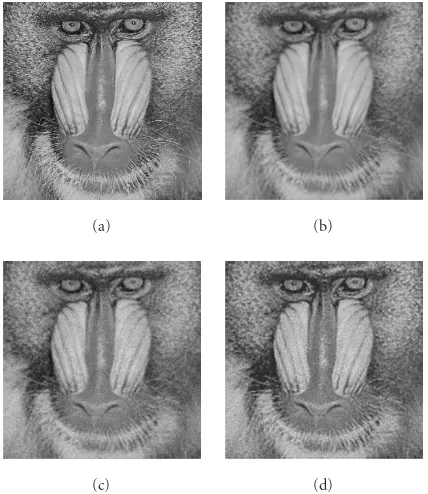
Figures7a,7b, and7cshow the original, blurred, and de-graded Lena images, respectively.Figure 7dshows the finally restored image by using Method B. Results for Baboon image are also shown inFigure 8. We can confirm the effectiveness of the proposed method.
5. IMAGE RESTORATION WITH VARIABLEγ
5.1. Determination ofγ
Natural images are composed of various components, such as the flat part and the edge. In order to efficiently remove noise components without degrading the image quality, we adjust the parameterγaccording to image characteristics in the cost function (20).
The new cost function with the variable parameterγ(xi) is represented by
J[F]= N2
i=1
yi−g
fi2
+ N2
i=1
γxifxi−N
+fxi−1
−4fxi+fxi+1+fxi+N2.
(23)
We should make the value of γ(xi) larger at the flat parts to efficiently remove noise components, and should make it smaller at the edges to preserve the edge information. We minimize J by using the steepest descent technique in the same way as (19), however the computation of∂J/∂ f(xi) is slightly different from the previous one. The detailed com-putation is shown inAppendix B.
(a) (b)
(c) (d)
Figure 7: Results for Lena image: (a) original image f(xi), (b)
blurred imageg(fi), (c) degraded imageyi, and (d) restored image
f(xi), (SNRI=1.82).
due to the increased effect of noise components. Therefore, we smoothed the test image by using the following mean fil-ter of size (3×3):
sxi=1 9
yi−N−1+yi−N+yi−N+1+yi−1+yi +yi+1+yi+N−1+yi+N+yi+N+1
,
(24)
and then estimated the edge position by the size of the deriva-tive ofs(xi), computed by
dxi=sxi−N
−sxi+N2+sxi−1
−sxi+12. (25)
The value ofd(xi) becomes small near the edges. We thus put
γxi=Ae−ad(xi) (26) so that the value ofγ(xi) becomes small near the edges, where
Aandaare constants. Equation (26) achieves a good tradeoff between restoration performance and computational sim-plicity, although other choices exist. We may estimate the edge position more accurately by using an order statistics fil-ter instead of the mean filfil-ter (24). But the use of the order statistics filter increases the computational complexity and the restoration performance is fairly robust against the value of the regularization parameterγ(xi) [16].
The restoration method with variable regularization pa-rameter is summarized as follows.
Step (1) We smooth the test image by the mean filter (24) to generate the edge imaged(xi), and then com-pute the value ofγ(xi) by using (26).
(a) (b)
(c) (d)
Figure8: Results for Baboon image: (a) original image f(xi), (b)
blurred imageg(fi), (c) degraded imageyi, and (d) restored image
f(xi), (SNRI=0.97).
Step (2) Using the training image, we initially estimate the blurring function by the GRBFN.
Step (3) Using the test image, we repeat the update proce-dure (19) 10 times to obtain a restored image at an intermediate stage.
Step (4) We regard the restored image as the original im-age, and again estimate the blurring function by using the test image.
Step (5) Repeat Step (3) and Step (4) until no significant improvement is attained in Step (3).
5.2. Restoration results
Figure 9shows the restoration results for Lena image, where we putA = 105anda = 0.05. These parameters were de-termined in a heuristic manner so that the SNRI becomes higher. Figures 9a,9b, and 9c show the smoothed images
s(xi), the edge image d(xi), and the finally restored image
f(xi). The value of SNRI is also shown. Results for Baboon image are shown inFigure 10. These results show that chang-ingγaccording to image characteristics improves the restora-tion performance by 0.25 (dB) and 0.39 (dB) for Lena and Baboon images, respectively.
(a) (b) (c)
Figure9: Results for Lena image with variableγ: (a) smoothed images(xi), (b) edge imaged(xi), and (c) restored image f(xi), (SNRI=
2.03).
(a) (b) (c)
Figure10: Results for Baboon with variableγ: (a) smoothed images(xi), (b) edge imaged(xi), and (c) restored imagef(xi), (SNRI=1.36).
6. CONCLUSION
We presented the nonlinear image restoration method by using the GRBFN and the regularization method. We used the GRBFN to estimate the nonlinear blurring function, and used the regularization method to restore the original image. We alternately used the two estimation methods for restor-ing the original image from the nonlinearly degraded image, under the single assumption of the smoothness of original image and blurring function. The salient feature is that the proposed estimation method is applicable even when the in-verse of the blurring process does not exist. We also presented the adaptive regularization parameter selection method for further improvement of restoration performance.
APPENDICES
A. COMPUTATION OF∂J/∂ f(xi)
The derivative ofJwith respect to f(xi) is represented by
∂J ∂ fxi =
∂ ∂ fxi
N2
j=1
yj−g
fj
2
+γ ∂ ∂ fxi
N2
j=1
fxj−N
+ fxj−1
−4fxj
+ fxj+1
+fxj+N2.
(A.1)
The first term in the right-hand side of (A.1) is expressed as
∂ ∂ fxi
N2
j=1
yj−g
fj2
=2 N2
j=1
yj−g
fj ∂
∂ fxi
yi−g
fj
= −2yi−N−1−g
fi−N−1
∂gfi−N−1
∂ fxi
−2yi−N−g
fi−N
∂gfi−N
∂ fxi
−2yi−N+1−g
fi−N+1
∂gfi−N+1
∂ fxi
−2yi−1−g
fi−1
∂gfi−1
∂ fxi
−2yi−g
fi∂g
fi
∂ fxi−2
yi+1−g
fi+1∂g
fi+1
∂ fxi
−2yi+N−1−g
fi+N−1
∂gfi+N−1
∂ fxi
−2yi+N−g
fi+N∂g
fi+N
∂ fxi
−2yi+N+1−g
fi+N+1
∂gfi+N+1
∂ fxi
(a) (b)
(c) (d)
Figure11: Results for a natural image: (a) original imagef(xi), (b)
blurred imageg(fi), (c) degraded imageyi, and (d) restored image
Here, (tj)ldenotes thelth element of the 9-dimensional vec-tor tj. The second term in the right-hand side of (A.1) is computed by
The derivative ofJwith respect to f(xi) is represented by
The first term in the right-hand side of (B.1) is computed by (A.2). The second term in the right-hand side of (B.1) can be computed by
∂ ∂ fxi
N2
j=1
γxj
fxj−N
+ fxj−1
−4fxj
+ fxj+1
+fxj+N2
=2γxi−N
fxi−2N
+ fxi−N−1
−4fxi−N
+fxi−N+1
+ fxi
+γxi−1
fxi−N−1
+ fxi−2
−4fxi−1
+ fxi+ fxi+N−1 −4γxifxi−N
+fxi−1
−4fxi
+ fxi+1+fxi+N
+γxi+1fxi−N+1
+ fxi−4fxi+1
+ fxi+2+ fxi+N+1
+γxi+Nfxi+ fxi+N−1
−4fxi+N
+ fxi+N+1+fxi+2N .
(B.2)
REFERENCES
[1] T. Poggio and F. Girosi, “Networks for approximation and learning,” Proceedings of the IEEE, vol. 78, no. 9, pp. 1481– 1497, 1990.
[2] J. Park and I. W. Sandberg, “Universal approximation using radial-basis-function networks,” Neural Computation, vol. 3, no. 2, pp. 246–257, 1991.
[3] F. M. A. Acosta, “Radial basis function and related models: an overview,”Signal Processing, vol. 45, no. 1, pp. 37–58, 1995. [4] B. Mulgrew, “Applying radial basis functions,” IEEE Signal
Processing Magazine, vol. 13, no. 2, pp. 50–65, 1996.
[5] S. Haykin, Neural Networks: A Comprehensive Foundation, Prentice Hall, Upper Saddle River, NJ, USA, 1999.
[6] D. Kundur and D. Hatzinakos, “Blind image deconvolution,”
IEEE Signal Processing Magazine, vol. 13, no. 3, pp. 43–64, 1996.
[7] M. R. Banham and A. K. Katsaggelos, “Digital image restora-tion,”IEEE Signal Processing Magazine, vol. 14, no. 2, pp. 24– 41, 1997.
[8] Y.-L. You and M. Kaveh, “A regularization approach to joint blur identification and image restoration,”IEEE Trans. Image Processing, vol. 5, no. 3, pp. 416–428, 1996.
[9] I. Cha and A. Kassam, “RBFN restoration of nonlinearly de-graded images,”IEEE Trans. Image Processing, vol. 5, no. 6, pp. 964–975, 1996.
[10] A. K. Katsaggelos,Digital Image Restoration, Springer-Verlag, New York, NY, USA, 1991.
[11] C. A. Micchelli, “Interpolation of scattered data: distance ma-trices and conditionally positive definite functions,” Constr. Approx., vol. 2, no. 1, pp. 11–22, 1986.
[12] S. Chen, C. F. N. Cowan, and P. M. Grant, “Orthogonal least squares learning algorithm for radial basis function net-works,” IEEE Transactions on Neural Networks, vol. 2, no. 2, pp. 302–309, 1991.
[13] A. Sherstinsky and R. W. Picard, “On the efficiency of the or-thogonal least squares training method for radial basis func-tion networks,”IEEE Transactions on Neural Networks, vol. 7, no. 1, pp. 195–200, 1996.
[14] S. Lee and R. M. Kil, “A Gaussian potential function net-work with hierarchically self-organizing learning,” Neural Networks, vol. 4, no. 2, pp. 207–224, 1991.
[15] A. G. Bors and M. Gabbouj, “Minimal topology for a radial basis functions neural network for pattern classification,” Dig-ital Signal Processing, vol. 4, no. 3, pp. 173–188, 1994. [16] N. P. Galatsanos and A. K. Katsaggelos, “Methods for
choos-ing the regularization parameter and estimatchoos-ing the noise variance in image restoration and their relation,” IEEE Trans. Image Processing, vol. 1, no. 3, pp. 322–336, 1992.
Keiji Icho received the B.E. and M.E. de-grees in communications engineering from Osaka University, Osaka, Japan, in 1999 and 2001, respectively. Since 2001, he has been working on software development for com-munication systems at Matsushita Electric Industrial Co., Ltd., Osaka, Japan.
Youji Iigunireceived the B.E. and M.E. de-grees in applied mathematics and physics from Kyoto University, Kyoto, Japan, in 1982 and 1984, respectively, and the D.E. degree from Kyoto University in 1990. He was an Assistant Professor at Kyoto Univer-sity from 1984 to 1995, and an Associate Professor at Osaka University from 1995 to 2003. Since 2003, he has been a Professor at Osaka University. His research interests in-clude signal and image processing.