R E S E A R C H
Open Access
Reduced-complexity FFT-based method for
Doppler estimation in GNSS receivers
Baharak Soltanian
1*, Ali Murat Demirtas
2, Ali Shahed hagh ghadam
3and Markku Renfors
1Abstract
In this article, we develop a novel algorithm for Doppler acquisition in fast Fourier transform (FFT)-based Global Navigation Satellite System (GNSS) receivers. The Doppler estimation is carried out in FFT domain by finding the frequency shift which maximizes the energy of the correlation vector. Subsequently, energy detection is used for preliminary decision about the presence of the target code. Then, the final decision and code phase estimation are done in the time domain after taking the inverse fast Fourier transform (IFFT). It is shown that the proposed algorithm has the potential for reducing the average number of required IFFTs in the acquisition process. For improving the sensitivity of the proposed approach, time-domain block averaging and FFT-domain non-coherent integration are investigated as alternative methods. They exhibit rather similar performance improvement, but the non-coherent integration approach is found to be computationally more effective.
Keywords: FFT-based acquisition; Energy detector; Doppler frequency estimation; GNSS receivers
1 Introduction
The direct-sequence spread spectrum (DSSS) technique is a method in which a signal of narrow bandwidth is intentionally spread over a wider bandwidth in the fre-quency domain. It provides security and lower sensitivity towards noise, interference, and jamming in communica-tion and posicommunica-tioning systems. Examples of systems using DSSS with code division multiple access (CDMA) are the Global Navigation Satellite Systems (GNSS), such as Global Positioning System (GPS) and Galileo.
In GNSS, the transmitter utilizes a pseudo random noise (PRN) sequence to expand a narrow-band signal over a wider spectrum. The PRN codes repeat with the period ofTc, and the codes used by different satellites
are quasi-orthogonal [1]. This means that the cross-correlation function between two different codes or the auto-correlation between a specific code and a shifted version of it takes a small value. A correlation peak is observed when taking a correlation between the received signal and a code which is present in the received sig-nal, and the two codes are aligned with each other [2,3].
*Correspondence: [email protected]
1Department of Electronics and Communications Engineering, Faculty of Computing and Electrical Engineering, Tampere University of Technology, Korkeakoulunkatu 10, 33720 Tampere, Finland
Full list of author information is available at the end of the article
If the carrier-to-noise ratio (CNR) is low, then the GNSS receiver must process more than a single code periodTc
of the received signal to find the code phase. Due to the unknown beginning of the PRN code in the received sig-nal, the code phase is a random variable with uniform distribution over a known interval which is the length of the PRN code. The length of the GPS Coarse/Acquisition (C/A) codes is 1,023 chips with Tc = 1 ms. The
com-mon approach to discover the code phase is to perform the correlation between the incoming baseband signal and a locally generated PRN code.
Another parameter which must be extracted by the receiver is the Doppler frequency shift caused by the satel-lite’s and the user’s motion. The Doppler frequency shift is also a random variable with uniform distribution over the interval of [−10, 10] kHz. The state of the art to estimate the Doppler frequency shift is that the receiver fulfills a sequential search over the interval of [−10, 10] kHz with a step size of α. The combination of search in the two dimensions for the code phase and the Doppler shift is called acquisition. The acquisition is performed either in the time domain, frequency domain, or combination of both [4-9].
The time domain acquisition is easy to implement on application-specific integrated circuit-based (ASIC)
devices, but it is time consuming when it comes to uti-lization of software-defined radio (SDR) receivers. Thus, a faster alternative for SDR-based devices is fast Fourier transform (FFT)-based acquisition which, however, has relatively high computational complexity.
The high complexity of the FFT-based acquisition is caused by (a) wide bandwidth of the incoming baseband signal which forces the device to deal with long FFT and inverse fast Fourier transform (IFFT) and (b) utiliza-tion of the convenutiliza-tional sequential search to estimate the Doppler frequency shift. The reason why GNSS receivers process wide bandwidth signal is to have sharper corre-lation peak and reduce the effect of multi-path. Having narrow bandwidth in acquisition stage rounds the cor-relation peaks for both direct and multi-path signals. Increasing the bandwidth of the signal is a solution for the mentioned problem, but it leads to high complexity due to the need of computing repetitive long FFTs and IFFTs [10].
An alternative solution for the sequential search is to employ optimum search methods such as binary search [11]. The challenge of long FFTs and IFFTs can be partly relaxed through the use of multi-rate signal processing [12].
In this paper, we address the problem of performing a large number of IFFTs while the receiver searches for the Doppler frequency shift. First, we propose utilization of maximum likelihood estimation in the FFT domain to find and estimate the Doppler shift. Then, we employ the concept of energy detection to determine the pres-ence of the desired signal in the frequency domain. This combination decreases the number of required IFFTs for FFT-based acquisition significantly. To the best of our knowledge, Doppler estimation in the FFT domain has not been elaborated in the GNSS literature.
In Section 2, the conventional FFT-based acquisition method is described. The FFT-based Doppler estimation algorithm is developed in Section 3. Numerical results and comparisons for GPS acquisition are presented in Section 4. Finally, our conclusions are given in Section 5.
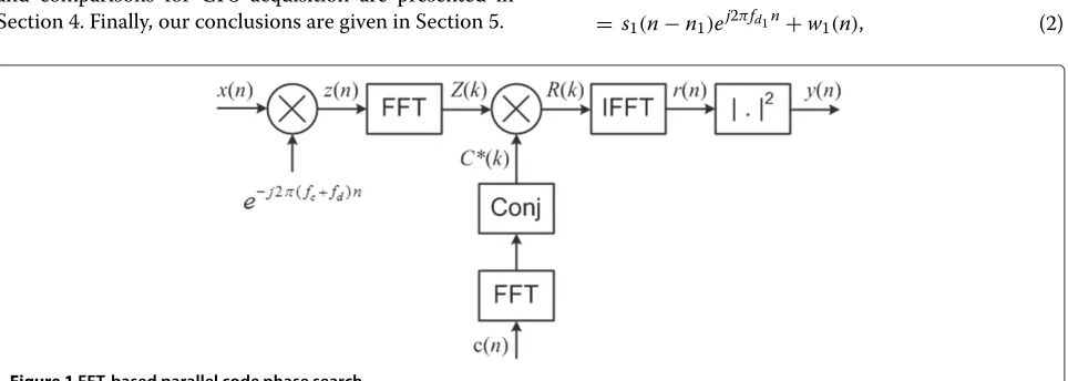
2 FFT-based acquisition algorithm
Figure 1 shows the block diagram of conventional FFT-based acquisition for GPS devices. First, carrier frequency is stripped off and the Doppler frequency shift is partially compensated, as explained later in Section 2.2. Afterward, the FFT of the incoming signal is multiplied by the conju-gate FFT of a locally generated PRN code. Finally, an IFFT is performed and a threshold test to find the peak of the auto-correlation function (ACF) is fulfilled. The drawback of this approach is high complexity due to repetitive long FFT and IFFT computations which increase the cost of the receiver.
2.1 Signal model
In this article, we assume that the channel is relatively flat fading for the bandwidth of the received signal and the GNSS signal we choose to deal with is GPS L1 signal. We model the received signal at baseband before Doppler removal as
x(n)= L
l=1
sl(n−nl)ej2πfdln+w(n), (1)
wheresl(n) = Alcl(n)dl andn ∈ [0,N−1] whereN is
the code length in samples. Here,Al,cl(n), anddlare the
gain, the PRN code, and the navigation data, respectively. The navigation data is assumed to be constant over the acquisition time interval. Note thatsl(n)is the transmitted
signal from thelth satellite andnlis the delay in samples, fdl is the normalized frequency shift due to the Doppler effect,L is the number of satellites in line of sight, and
w(n)is additive white Gaussian noise withEs2l(n) Ew2(n). Thus, it is possible to assume that eachs
l(n)
is a wide-sense stationary (WSS) Gaussian process [2]. For simplicity, we rewrite the incoming baseband signal as follows:
x(n) = s1(n−n1)ej2πfd1n+
L
l=2
sl(n−nl)ej2πfdln+w(n)
= s1(n−n1)ej2πfd1n+w1(n), (2)
wheres1(n)is the target satellite signal,sl(n)denotes the
received signals from other satellites in line of sight, and
w1(n) = L
l=2sl(n−nl)ej2πfdln+w(n)is the noise plus
interference term.
2.2 Circular correlation and Doppler estimation
The circular correlation between the incoming baseband signal after partial Doppler removal,z(n), and the corre-sponding real spreading codec1(n)can be expressed as
r(n) = N
where fl is the normalized frequency offset after car-rier plus partial Doppler removal,r1,1(n)is the correlation function of the target signal, andu(n) = Ll=2r1,l(n)+ u1(n). This can be expressed in the frequency domain as
R(k) = Z(k)×C∗1(k)
= R1,1(k)+U(k). (4)
It follows that frequency shifts which are multiples of the FFT resolution (FFT bin spacing) can be imple-mented through shifting the FFT of the input signal. If this resolution is not sufficient in the Doppler search, then improved resolution can be reached by taking the FFT for the received baseband signal with partial Doppler removal. In the GPS case, the FFT resolution is commonly 1 kHz, while 500-Hz Doppler resolution is targeted at the acquisition stage.
The frequency interval in which the Doppler frequency shift belongs to is known to the receiver. It is commonly assumed to include also the GPS receiver’s local oscillator frequency offset and selected as [−10, 10] kHz. Conven-tionally, in order to estimate the Doppler effect in the FFT-based receiver, a sequential search over the interval of [−10, 10] kHz with a step size ofα = 0.5 kHz is per-formed. For each candidate Doppler frequency, the FFT of the resultant signal is multiplied by the conjugate FFT of a locally generated PRN code and an IFFT is computed. In the worst case, the receiver has to perform FFT forβ =
20
0.5+1=41 shifted versions of the input signal and multi-ply the resultant signal each time by the conjugate FFT of the PRN code. Then, it is needed to computeβIFFTs and search for the peak of the correlation function for each of them. Since the FFT bin spacing is 1 kHz, the FFTs with Doppler values of −10,−9,−8,. . ., 10 kHz can be
obtained from a single FFT just by shifting the FFT bins. Likewise, the Doppler cases of−9.5,−8.5,. . ., 9.5 kHz can be obtained from a single FFT with 0.5-kHz shift imple-mented before FFT. Consequently,β+2 FFTs/IFFTs are needed altogether to test all possible Doppler values.
The conventional algorithm is as follows:
Conventional algorithm
1. Strip off the carrier frequency and take the FFTs of the incoming signal and its 500-Hz shifted version. 2. Perform the conjugate FFT of the locally generated
PRN code.
3. ForDoppler= −10 : 0.5 : 10kHz
(a) Shift FFT of the incoming signal to compensate the Doppler frequency shift. (b) Multiply the resultant signal from step 3a by
the final result from step 2.
(c) Take the IFFT of the outcome of step 3b. (d) Find the acquisition margin (AM).
(i) IfAM> γ, then terminate.
End End of algorithm
Here, AM is the ratio of the maximum of the magnitude of the correlation function to its second maximum peak.
The drawback of conventional approach is that the receiver needs to performβ = 41 times IFFT of length
N = fsTcin the worst case. HerefsandN are the
sam-pling frequency and the FFT length, respectively. This increases the complexity of the system in comparison to time-domain acquisition, and in this paper, our goal is to overcome the problem by introducing a new algorithm.
3 Proposed algorithm
Due to the complexity caused by the widely implemented method of FFT-based acquisition, a big challenge is how to reduce the complexity of the overall system. One of the items that increases the complexity is the utilization of the sequential search method to attain the Doppler fre-quency shift. As mentioned, in the worst case,β+2=43 FFT/IFFT transform calculations are needed.
false alarm probabilities, is sufficient in such FFT-domain acquisition.
Our proposed algorithm divides the acquisition stage into three steps: (a) estimate the Doppler frequency shift in the frequency domain, (b) compare the decision vari-able against a threshold to check whether the signal of interest is present, and (c) find the related code phase.
In the next subsections, first we describe the effect of the Doppler frequency shift on the acquisition stage. Then, we explain how to search for the Doppler in the frequency domain and finally how to utilize the energy detector and set the threshold to detect the presence of the desired signal.
3.1 Doppler frequency shift
One of the parameters that must be estimated in the acquisition stage is the Doppler frequency shift which is caused mainly by the Doppler effect resulting from the satellite’s and the user’s motion. It is a random vari-able with a uniform distribution over [−10, +10] kHz. The residual frequency offset has two effects: (a) it atten-uates the correlation function’s (CF) peak value signif-icantly, and (b) it may cause fractional chip shift [13]. This is the reason why the GPS receiver must estimate the Doppler frequency shift with a reasonable error/offset [14]. Typically,±250 Hz residual frequency offset range is considered acceptable at the acquisition stage.
Ignoring the noise plus interference terms, the cross-correlation function (CF) between the incoming signal and the code sequence after the partial Doppler and the carrier removal is
ρl(nl−ml)= N−1
m=0
Aldlcl(nl+m)ej2πflm×cl(ml+m), (5)
wherenlis the incoming signal’s code phase,mlis the PRN
code’s code phase, andfl is the residual frequency off-set. The maximum magnitude of the CF happens when the code phases are completely aligned. This meansnl =ml.
ρl(0)= N−1
m=0
Aldl|cl(m+nl)|2ej2πflm. (6)
It can be assumed thatdlis constant over 1 ms of
corre-lation time, and sinceci(m+nl)is a sequence of±1, then
Equation (7) can be used for evaluating the effect of a given Doppler shift on the acquisition performance. It shows that the Doppler shift affects the CF’s peak in two ways: First, it introduces an exponential term of
ejπfl(N−1)which is a constant phase rotation. Second, the term sin(πflN)/sin(πfl), attenuates the magnitude of the CF and may jeopardize the correlation process [13,15]. Thus, before checking whether the signal is present, it is necessary to estimate the Doppler frequency shift with sufficient resolution.
3.2 Doppler search in the frequency domain
The following analysis is based on the model that the FFT input z(n) is the received baseband signal after carrier and partial Doppler removal andc1(n)is the target PRN code. The noise is assumed to be additive complex cir-cular white Gaussian (AWG) with distributionN(0,σ2). If the received signal is WSS and its length is sufficiently large, then the maximum likelihood estimate (MLE) can be found by minimizing [16]
J(kd)=
where k is the FFT index, kd is the trial Doppler, Pzz(k;kd) = Zzz(k−kd)+Zzz(−k+kd) andZzz(k) = |Z(k)|2is a low-pass power spectral density (PSD) of the FFT input signal,z(n), andI(k)is the periodogram of the target PRN code. SinceNk=−Nln depend onkd, then the ML solution can be simplified as
T1(s1)=max
Because the GPS power spectrum is clearly below the noise spectrum, the ML solution can be written as follows:
T2(s1)=
If we substitute (9) into (11), then
Ignoring the non-essential constant multiplier, we obtain
Equation (14) suggests performing a grid search in the frequency domain over the interval of [−10, +10] kHz in order to find the frequency offset which gives the highest energy in the frequency domain. For the energy grid search (EGS), the required number of FFT/IFFTs is
Nr =3, while for the conventional search, the number of
required FFT/IFFTs isNr = β+2. The price to be paid
for reducing the required number of FFT/IFFTs is lower probability of detection for weak signals.
One approach to solve the mentioned problem is to per-form the IFFT for the Doppler frequency shift which gives the maximum energy for EGS and checks whether the correlation function’s peak in the time domain is observ-able. If true, then terminate the search; otherwise, move to the Doppler frequency which gives the second maximum value and continue till the peak of correlation function is detectable.
3.3 Signal detection in the frequency domain
In the previous subsection, we explained how to search for the Doppler frequency shift in the frequency domain. Equation (14) shows that the maximum likelihood esti-mation of the Doppler frequency shift resembles energy detection.
In spite of the significant saving on the required num-ber of IFFTs, the plain concept of the EGS for low CNR demonstrates low probability of detection compared with the conventional search. We modify our algorithm in order to overcome the mentioned drawback. Each time the receiver checks the maximum energy in the fre-quency domain to confirm whether the correct Doppler frequency shift is found, it performs the IFFT. If the cor-rect Doppler frequency is not found, then the receiver moves to the next Doppler frequency which gives the sec-ond maximum in the energy and the search is terminated if the correct Doppler shift is found. By this, the probabil-ity of the detection improves. This approach has one more drawback. In the absence of the desired signal, the receiver must performβ IFFTs which increases the complexity of the proposed algorithm. To address this problem, we pro-pose the utilization of the energy detector in the frequency domain to check whether the desired signal is present.
The notion of the energy detector has been used in many different areas of signal processing, and in the recent decade, it has been applied extensively in cognitive radios [17].
The theory of energy detection starts by defining the null and the present hypotheses which in our case are as follows:
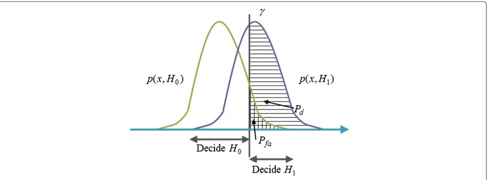
H0:r(n)=u(n), n=1, 2,· · ·,N, (15a) H1:r(n)=r1,1(n)+u(n), (15b)
whereH0andH1are the null and present hypotheses as shown in Figure 2,r1,1(n)is the correlation function of the target signal, andu(n)is noise plus the cross-correlation functions for the signals of other satellites in line of sight. The decision statistic is
T = 1
SinceN, the length of the received signal, is sufficiently large, it is possible to assume thatT has a normal distri-bution of
The probability of detection,Pd, and probability of false
alarm,Pfa, can be calculated from
Pfa = Q
whereγ is the detection threshold.
In order to detect the signal in the frequency domain, it is possible to utilize the Parseval theorem as follows:
T =N
This means that the total energy of a signal in both time and frequency domains are equal [18].
In the energy detector, the threshold depends on the power of the noise so it must be either known or possible to estimate. In the case of GNSS signals, the noise after the correlation stage, Equation (3), contains two parts: (a) the thermal noise,w(n), caused by the receiver itself and (b) the cross-correlation functions due to the presence of the other satellites,Ll=2r1,l(n). The first part can be
estimated, but the second part is difficult if not impossi-ble, and that is the source of the noise uncertainty in the utilization of the energy detector for the GNSS receiver. The effect of the uncertainty on the estimation of the noise introduces a limit on the performance of the energy detector [19,20].
Figure 2Probability density functions for signal plus noise and plain noise.
input signal with an unused PRN code [5]. In our simula-tions, the unused PRN is chosen as code number 32. Then, the interference plus noise power can be estimated as
σ2
We can assume that the noise is uncorrelated with the code. Then, it follows that
σ2
e is the power estimated with the unused PRN
code and σ2
u is the variance of the thermal
noise-dependent part of the correlation. By substituting (20) in (17),
and the threshold,γ, is calculated as
γ =
After we determine an approximation of the power of noise using Equation (20), we then are able to use Equation (22) to calculateγ.
In Equation (22), the first term,Ll=1σ32,2 l1+Q−1Pfa
/ √
N, has a critical role when it comes to the matter of choosingγ. If there are no interference signals from other satellites, to chooseγ, two parameters have to be consid-ered, Pfa and σu2; the lower thePfa, the higher γ which
leads to lower Pd. In our case, when there is
interfer-ence from other satellites in line of sight (LOS), the term L
l=1σ32,2 l does not present the real value of the
inter-ference’s power. Then, we do face an error (bias value) in our estimation, and we have to choose γ and Pfa
very conservatively which results in higherPfaand lower γ [16].
Using PRN number 32 to estimate the noise power introduces an errorσ2. If we use the desired PRN code instead of the PRN code 32, then
σ2
whereσu2is again the thermal noise-dependent part and
σ2
1,l are the powers of the actual auto/cross-correlation
functions. Then, the error or the noise uncertainty is
to be processed. As a result, noise uncertainty introduces an SNR wall which is derived in [19] as follows:
SNRwall= ρ 2−1
ρ , (24)
whereρ=1+σ2/σr2.
Equation (23) shows that the noise uncertainty in GNSS receivers is caused by the number of satellites in line of sight, their power levels, and the cross-correlations between corresponding PRN codes and the target code and the unused code.
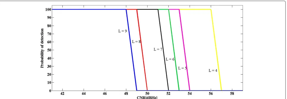
Figure 3 shows the effect of the power of other satellites in line of sight. As we predict, the lower the number of the satellites in line of sight,L, the better the probability of de-tection. The target PRN is PRN number 2 with a CNR of 52 dB-Hz,L∈[4, 9] is the number of satellites in line of sight, and all the other satellites in line of sight have equal CNR. Here, we choose thePfa=65% to calculateγusing Equation
(22). Due to the uncertainty in calculating the power of the noise, we have to choose thePfahigher than usual.
3.4 Final algorithm
In subsections 3.2 and 3.3, we explained the search algo-rithm for the Doppler frequency shift and the detection procedure for the desired signal. As we mentioned, the problem with the plain EGS is that in spite of significant saving on the number of required IFFTs for strong signals, the algorithm’s performance for weak signals is not as good as the conventional approach. To solve the problem, we modified the search algorithm in order to be competitive with the conventional search, but this approach has a drawback. If the signal of interest is absent, then the receiver must go through the search list and performβ IFFTs. To deal with the mentioned problem, we employ an energy detector to detect the presence of the desired signal.
The final algorithm can be summarized as follows:
Proposed algorithm
1. Strip off the carrier frequency and take the FFTs of the incoming signal and its 500-Hz shifted version. 2. Perform the conjugate FFT of the locally generated
PRN code.
3. ForDoppler= −10 : 0.5 : 10kHz
(a) Shift FFT of the incoming signal to compensate the Doppler frequency shift. (b) Multiply the resulting signal from step 3a by
the final result from step 2.
(c) Calculate the energy of correlation function resulting from step 3b.
End
4. Find the highest energy,Emax, from step 3c in the
frequency domain.
5. Initiate the countercount=0
6. While(Emax> γ)&&(β >count)
(a) Take IFFT of the resultant signal. (b) Check the peak of correlation function. (c) IfThe peak is detectable
(i) Terminate the search (d) Otherwise
(i) Find the next highest energy of the energy from step 3c in the frequency domain. (ii) Increase the countercount+ +.
End
End End of algorithm
Here, β is the maximum number of required IFFTs, which in our case is 41.
3.5 Coherent block averaging
In the previous subsection, we explained our proposed algorithm. We mentioned that the EGS is sensitive to the power of interfering signals from other satellites in LOS. To overcome this problem, we consider utilizing block averaging (BA) to enhance the power of the desired signal [21]. Block averaging means processing B non-overlapping blocks with the length of 1 ms (code epoch) and adding them together.
xB(n)= B−1
i=0
x(n+iN), (25)
where 0 ≤ n < N,N is the number of samples in 1 ms of signal, andBis the number of milliseconds to be block averaged, respectively.
Substitutingx(n)=c(n)d(n)ejπfdninto (2) results in
xB(n)= B−1
i=0
c(n+iN)d(n+iN)ej2πfd(n+iN). (26)
Since for the C/A codec(n+iN)=c(n)andd(n)can be assumed to be constant over averaging timeB≤20 ms, it is possible to rewrite (26) as follows:
xB(n)= B−1
i=0
c(n)d(n)ej2πfdnhf
d(B), (27)
where
hfd(B)=
B−1
k=0
ej2πfdk= 1−e
j2πfdB
1−ej2πfd (28)
is the block-averaging gain function.
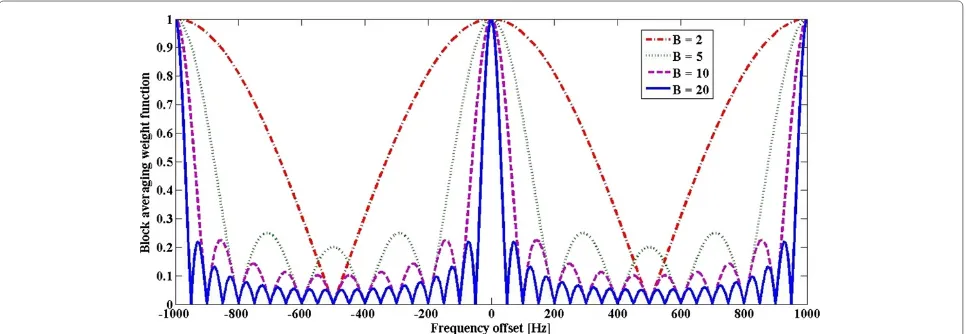
As Figure 4 shows, when BA is utilized, the frequency offset must be lower than 250 Hz. In order to be able to benefit from BA, we have to choose a step size of much
less than 500 Hz, which increases the number of required FFTs.
3.6 Non-coherent integration
Another alternative to enhance the power of the incoming signal is utilization of non-coherent integration in the FFT domain. We take B milliseconds of consecutive incom-ing signal and transfer each millisecond individually into the frequency domain, and finally, we take sample-wise squared magnitudes of theBFFTs and average them. By this, the required number of transforms remains the same but the number of Doppler values in the search is reduced considerably, compared to BA with the same length.
4 Analysis, numerical comparison, and result In this section, numerical and statistical results of our proposed algorithm are presented.
4.1 Numerical results
In our simulation study, we use GPS L1 frequency of 1,575.42 MHz, C/A code of length 1,023 chips, chip rate of 1.023 MHz, and oversampling factor of 8. In this case, a timing error of one chip corresponds to about 300 m error in pseudorange. Conventionally, in acquisition stage, the target for timing error is±0.5 chips.
In the signal of Equation (2),L= 6, and we choose the PRN codes 1 to 6 to be used. The target code is number 2, and its CNR is in the range of [36, 59] dB-Hz. The average CNR from other satellites in LOS is 41 dB-Hz. In our case, they are as [39, 42, 36, 45, 40].
Figure 5 shows the probability of detection for both the EGS and the conventional search for Doppler frequency. For each CNR∈[49· · ·59] dB-Hz, we run our simulation 500 times to find the probability of detection. As it was mentioned, the required number of FFT/IFFT for EGS is 3, while for conventional Doppler frequency search, the
Figure 5Probability of detection.For conventional search for Doppler frequency and for the FFT-domain grid search based on maximum energy (without time-domain peak detection).
required number of FFT/IFFT isβ+3 in the worst case. The price that we pay for the significant saving on IFFTs is low probability of detection for weak signals. To overcome the problem, we propose that after finding the maximum energy, the receiver performs an IFFT and checks for the correlation function’s peak. If it is detectable, the search is terminated; otherwise, the next local maximum value of the energy is checked, and the search is continued till the peak of the correlation function is visible.
Our initial approach has a drawback when the desired signal is absent. In the absence of the desired signal, the receiver has to perform an IFFT for each Doppler value included in the search. We propose utilizing an energy detector in order to solve the mentioned problem. The receiver checks whether the desired signal is present or not using a threshold determined from the target CNR and detection probability. Since the receiver calculates the
energy of the correlation function while it searches for the Doppler frequency shift, thus using the energy detector will not increase the complexity of the algorithm.
Figure 6 shows the average number of the required IFFTs for both conventional and proposed final algorithm when the desired signal is absent. The number of required IFFTs for our proposed algorithm is about half of the conventional approach on the average.
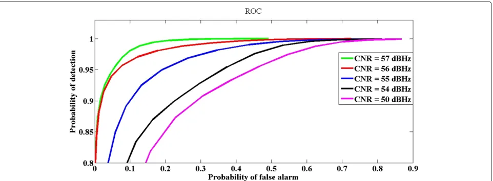
Figure 7 shows the receiver operating characteristic (ROC) for different CNRs when using the proposed method for estimating the interference plus noise power based on correlation with the unused PRN code. Figure 8 shows the ROC curves in the ideal case when there is no uncertainty in the interference plus noise estimation. These results indicate clearly that improved estimation of the interference plus noise power would greatly enhance the performance of the proposed approach. Since there is
Figure 7ROC for the energy detector utilizing proposed unused PRN correlation method for estimating interference plus noise power.
a trade-off between the threshold,γ, and the probability of false alarm,Pfa, if we take 50 dB-Hz as the target CNR
andPd=99% as the target detection probability, then the
threshold should be selected in such a way that the false alarm probability becomesPfa=0.65.
Figure 9 shows the ROC curve when the GPS receiver processes 10 ms of incoming signal by BA. It exhibits that if the target CNR > 44 dB-Hz and the target probability of detection is 99%, then the threshold should be selected in such a way that the false alarm probability becomes
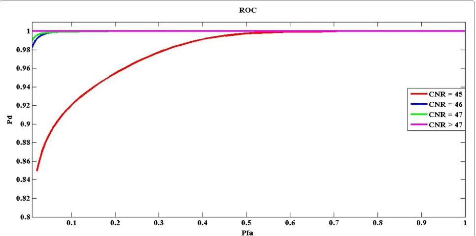
Pfa=0.5. Figure 10 displays the ROC curve when the GPS
receiver utilizes the EGS plus non-coherent integration when 10 ms of incoming signal is processed. If the target CNR > 45 dB-Hz and the target probability of detection is 99%, then the threshold should be selected in such a way that the false alarm probability becomesPfa=0.5.
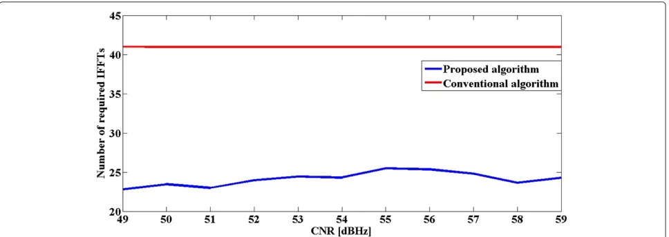
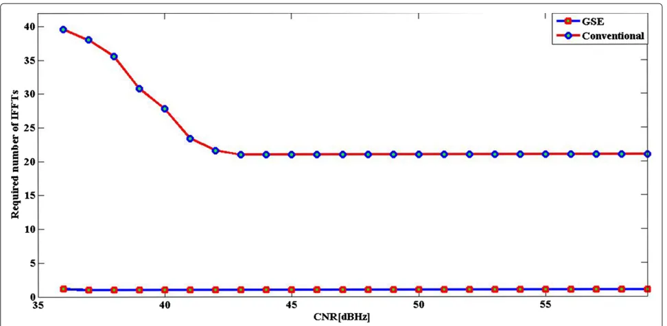
Figure 11 shows the result for our basic solution processing GPS signal over 1 ms interval. We can
observe that the number of the required IFFTs on average for our proposed algorithm is significantly less than the number of required IFFTs for conventional search. The probability of detection is the same for both approaches.
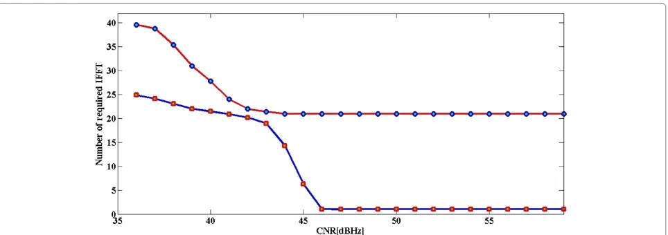
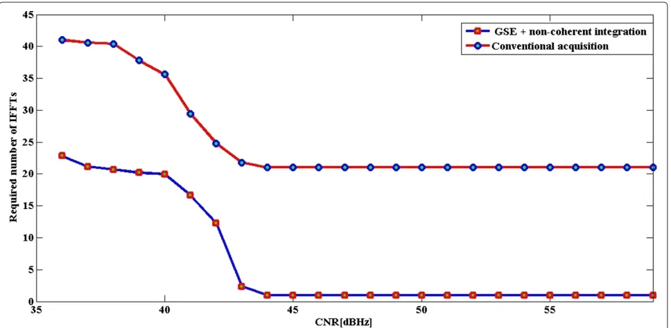
Figures 12, 13, 14 show the result when block aver-aging over 5, 10, and 20 ms of the incoming baseband signal is utilized. The result demonstrates an improve-ment for weak signals. Particularly, BA over 20 ms reduces the number of required IFFTs significantly. In Figure 15, the result for non-coherent integration over 10 ms is also shown.
4.2 Complexity comparison
In this subsection, we compare the complexity of the proposed algorithm with conventional FFT-based acqui-sition. As complexity metric, we use the number of real multiplications needed in the acquisition process.
Figure 9ROC for the energy detector when 10 ms of signal is block averaged.
With the oversampling factor of 8, FFT/IFFT lengths of N = 8, 192 are used, and each transform takes
N(log2(N)+3)+4=131, 076 real multiplications when using the efficient split-radix algorithm. This can be well approximated as 16Nreal multiplications. Table 1 shows the number of required FFTs for different approaches. Note that when the BA is utilized, the frequency offset after Doppler removal must be less than 50 Hz forL=10. The FFT-domain decision variable can be calculated asNk=−01|Z(k−kd)|2×C∗1(k)
2
whereZ(k−kd)is the
shifted version of the incoming baseband signal andkd ∈
[−10, +10]. The squared magnitude FFT vectors for dif-ferent codes can be pre-calculated and stored. In the basic
EGS algorithm and with non-coherent integration (NCI), the squared magnitude FFT vector for the input needs to be calculated twice, for the 0- and 500-Hz offsets. With coherent block averaging ofNBA1 ms intervals, this num-ber becomes 2NBA. The same FFTs and the same squared magnitude vectors are used for acquisition of all codes, so the effect of these calculations on the overall com-plexity is relatively small. What needs to be calculated intensively is the product of the squared magnitudes for each tested Doppler value. This takesN real multiplica-tions for each Doppler test, if all the FFT bins are used. To cover all the Doppler cases,(40NBA+1)Nreal multiplica-tions are needed, which have about the same complexity
Figure 11Required IFFTs.Number of required IFFTs on the average when 1 ms of received signal has been processed for conventional search and for iterative EGS with time domain peak detection. The probability of detection for both approaches is 99%.
as 2.5NBAIFFTs. The conventional FFT-based algorithm uses a multiplication of two complex vectors of length
N in the FFT domain, which is assumed to take 3N real multiplications.
Table 1 shows detailed comparison of the complexity of different FFT-based acquisition schemes. The number of real multiplications is given in two parts: The first part is independent of the number of different codes (C) cov-ered in the search, and the second part is proportional to
C. The ‘high CNR’ cases of Table 1 are cases where the correlation peak can be reliably detected in the frequency domain by the EGS method and in the time domain by the traditional approach. ‘Low CNR’ cases of the table corre-spond to the the situation where the code is not detectable anymore.
Due to the increased number of Doppler values to be tested, the coherent block averaging seems to be less efficient than the non-coherent integration approach. However, the complexity of the algorithm can be greatly reduced by doing the FFT domain multiplications only for the strong FFT bins of each code. Furthermore, it might be preferable to change the search strategy while con-sidering all the PRN codes that can be expected to be present in the received signal. An alternative approach is to try to find the strongest codes first, without iter-ating the time-domain peak checking. This can be done by testing the highest FFT-domain energy cases for all possible codes, before going to the iterative peak detection. These ideas remain as a topics for further studies.
Figure 13Required IFFTs.Number of required IFFTs on the average when 10 ms of received signal has been processed for iterative EGS with coherent BA and 1 ms of signal processed for conventional approach with time domain peak detection. The probability of detection for both approaches is 99%.
5 Conclusion
In this article, we propose a novel approach for FFT-based acquisition in GNSS receivers. Our approach contains uti-lization of both the EGS and the energy detector together. We use the EGS to estimate the Doppler frequency shift in FFT domain. Employing the EGS only causes a problem
when the target signal is not present as the device must perform IFFTs for all the Doppler values included in the search before it is able to terminate the search. To solve this problem, we employ an energy detector aiming to detect the presence/absence of the desired incoming baseband signal in the frequency domain.
Figure 15EGS plus non-coherent integration over 10 ms in comparison to conventional FFT-based acquisition.
To improve the sensitivity, coherent block averaging methods in the time domain and non-coherent inte-gration methods in the FFT domain were tested. The performance of these two approaches turned out to be rather similar, but the FFT-domain non-coherent integra-tion method has significantly lower complexity. For 10-ms noncoherent integration, with CNRs at or above 43 dB-Hz, the Doppler could be estimated in the FFT domain reliably, requiring only one or two IFFTs for the acqui-sition. With lower CNRs, the number of required IFFTs grows rapidly, approaching 50% of the Doppler values with very low CNR or in the absence of the PRN. For exam-ple, when searching over 20 PRN codes out of which 4 are present at around 43 dB-Hz level, the complexity in terms of real multiplications is reduced by about 40% compared
to the traditional FFT-based methods with 1-ms time interval.
In our future work, the main issue is improving the reli-ability of the detection of the presence/absence of PRN codes in the FFT domain. We will address the noise uncertainty and its effect on the performance of the pro-posed algorithm by trying to find improved methods for estimating the interference plus noise variance. We also plan to investigate the possibility of using a sub-stantially smaller number of strongest FFT bins, as well optimized search strategy considering all the possible PRN codes. In addition, we will substitute the conven-tional linear search for the modified binary search while we search for the Doppler frequency shift and observe the effect.
Table 1 Complexity evaluation of different FFT-based acquisition schemes
Algorithm Number of FFTs Number of tested Average number Number of real
Doppler values of IFFTs multiplications
High CNR Low CNR High CNR Low CNR
Conventional FFT-based 2 41 20.5 41 32N+390CN 32N+780CN
EGS (1 ms) 2 41 1 25 36N+57CN 36N+441CN
EGS + BA (5 ms) 10 201 1 25 180N+217CN 180N+601CN
EGS + BA (10 ms) 20 401 1 25 360N+417CN 360N+801CN
EGS + BA (20 ms) 40 801 1 25 720N+817CN 720N+1, 201CN
EGS + NCI (10 ms) 20 41 1 25 322N+57CN 322N+441CN
Competing interests
The authors declare that they have no competing interests.
Author details
1Department of Electronics and Communications Engineering, Faculty of Computing and Electrical Engineering, Tampere University of Technology, Korkeakoulunkatu 10, 33720 Tampere, Finland.2Center for Pervasive Communications and Computing, Electrical Engineering and Computer Science, University of California Irvine, Irvine, CA 92697-2625, USA.3Maxlinear, 2051 Palomar Airport Rd., Carlsbad, CA, USA.
Received: 24 December 2013 Accepted: 20 August 2014 Published: 15 September 2014
References
1. T Nighswander, B Ledvina, J Diamond, GPS software attacks, in19th ACM Conference on Computer and Communications Security, CCS 2012, Raleigh, NC, USA,(16–18 Oct 2012)
2. CW Therrien,Discrete Random Signals and Statistical Signal Processing. (Prentice Hall, Upper Saddle River, NJ, USA, 1992)
3. P Misra, P Enge,Global Positioning System. Signal, Measurements and Performance, Second Edition. (Ganga-Jamuna Press, Lincoln, MA, USA, 2006)
4. DJR van Nee, AJRM Coenen, New fast GPS code-acquisition technique using FFT. Electron. Lett.27(2), 158–160 (1991)
5. ED Kaplan, CJ Hegarty,Understanding GPS: Principles and Applications, 2nd edn. (Artec House, Norwood, MA, USA, 2005)
6. XL Cao, RZ Mu, YP Yan, A novel threshold setting method for FFT-based GPS acquisition, in11th International Conference on Computer Modelling and Simulation, 2009. UKSIM ’09, Cambridge, UK, (2009), pp. 497–501 7. Y Zheng, A software-based frequency domain parallel acquisition
algorithm for GPS signal, in2010 International Conference on Anti-Counterfeiting Security and Identification in Communication (ASID), Chengdu, China, (18–20 July 2010), pp. 298–301
8. R Davenport, FFT processing of direct sequence spreading codes using modern DSP microprocessors, inNational Aerospace and Electronics Conf, Dayton, OH, USA, (20–24 May 1991)
9. D Akopian, Fast FFT based GPS satellite acquisition methods. Radar Sonar Navigation IEE Proc.152(4), 277–286 (2005)
10. T Kos, I Markezic, J Pokrajcic, Effects of multipath reception on GPS positioning performance, inInternational Symposium ELMAR, Zadar, Croatia, (15–17 Sept. 2010)
11. B Soltanian, M Demirtas, M Gabbouj, Reduced-complexity binary search for Doppler estimation in GNSS receivers, in47th Asilomar Conference on Signals, Systems and Computers, (3–6 Nov. 2013)
12. B Soltanian, J Collin, J Takala, The effect of the incoming signal decimation on the performance of the FFT-based acquisition stage in SDR GNSS receivers, in5th ESA Workshop on Satellite Navigation Technologies (NAVITEC), Noordwijk, Netherlands, (8–10 Dec. 2010) 13. J Tsui,Fundamentals of GPS Receivers: A Software Approach. (John Wiley &
Sons, Inc., New York, USA, 2002)
14. K Borre, DM Akos, N Bertelsen, P Rinder, S Jensen,A Software-Defined GPS and Galileo Receiver - A Single-Frequency Approach. (Birkhauser, Boston, 2007)
15. L Dai, Z Wang, J Wang, J Song, Joint code acquisition and Doppler frequency shift estimation for GPS signals, inVehicular Technology Conference, (2010)
16. SM Kay,Fundamentals of Statistical Signal Processing Volume II Detection Theory. (Prentice-Hall, Upper Saddle River, NJ, USA, 1993)
17. ATD Cabric, R Brodersen, Spectrum sensing measurements of pilot, energy, and collaborative detection, inIEEE Military Commun. Conf. (MILCOM), Washington D.C., USA, (23–25 Oct. 2006)
18. RW Schafer, JRB Alan, V Oppenheim,Discrete-Time Signal Processing. (Prentice-Hall, Upper Saddle River, NJ, USA, 1998)
19. R Tandra, A Sahai, SNR walls for signal detection. IEEE J. Selected Topics Signal Process.2(1), 4–17 (2008)
20. R Tandra, A Sahai, Fundamental limits on detection in low SNR under noise uncertainty, inInternational Conference on Wireless Networks, Communications and Mobile Computing, Maui HI, USA, (13–16 June 2005) 21. M Sahmoud, MG Amin, R Landry, Acquisition of weak GNSS signals using
a new block averaging pre-processing, inIEEE/ION Position, Location and Navigation Symposium, Monterey, CA, USA, (5–8 May 2008)
doi:10.1186/1687-6180-2014-143
Cite this article as:Soltanianet al.:Reduced-complexity FFT-based
method for Doppler estimation in GNSS receivers.EURASIP Journal on Advances in Signal Processing20142014:143.
Submit your manuscript to a
journal and benefi t from:
7Convenient online submission 7Rigorous peer review
7Immediate publication on acceptance 7Open access: articles freely available online 7High visibility within the fi eld
7Retaining the copyright to your article