R E S E A R C H
Open Access
Research on time difference detection
algorithm based on combination of GNSS
and PPP
Jun Yang
1, Ziwen Zhang
2*, Yijun Liu
2, Zuoteng Xu
2, Haowen Chen
2, Wende Zhang
2and Yuqiang Chen
3Abstract
With the gradual increase in the number of GNSS systems and the improvement of functions, in addition to the single-system navigation and timing service, the integrated navigation and positioning service among multiple single-systems can provide users with more accurate and stable positioning results, arousing more attention from the workers in GNSS field. Compatibility and interoperability among different systems has become a trend in the development of GNSS. Compatibility and interoperability between systems require a uniform time scale. Therefore, the measurement and forecasting of time deviations in GNSS systems is particularly important. This paper first studies the multi-system fusion location model and proposes an adaptive GNSS fusion PPP algorithm based on parameter equivalent reduction. Then, the method of fusion PPP is used to monitor the time difference of GNSS. Finally, the effectiveness of the improved algorithm and time difference monitoring method is verified by practical examples.
Keywords:GNSS, PPP algorithm, Pseudo-time difference, Time difference monitoring
1 Introduction
The official launching of China’s Beidou second-generation satellite navigation system indicates that the number of glo-bal satellite navigation and positioning systems (GNSS) cur-rently providing services has increased from two to three. The number of GNSS working satellites has exceeded 70. In the next 5 to 10 years, with the completion of the EU Galileo system, the total number of GNSS satellites will exceed 100, and the vast majority are modern multi-frequency oper-ational satellites. GNSS has entered a new chapter of multi-constellation and multi-frequency [1]. With the modernization of GNSS, the timing accuracy of multi-system integrated navigation positioning is also increasing. The de-velopment characteristics of GNSS have also gradually chan-ged from the single GPS positioning model that initially focuses on post-processing relative positioning to the multi-system GNSS fusion absolute positioning with fast real-time and high-frequency observations. Among them, the rapid and flexible precision point positioning technology
(PPP) is undoubtedly one of the most promising application technologies [2].
The accuracy and stability of real-time fast positioning will be greatly improved by using the fusion and posi-tioning of GNSS multi-system. In recent years, the re-search results of GNSS fusion PPP both at home and abroad are more abundant, mainly concentrated in the [3] GPS/GLONASS fusion. For example, Dr. Kuang of JPL proposed that the precision orbit of GLONASS sin-gle star or constellation could be determined based on the space-time system of the GPS system, and the orbit determination accuracy of GLONASS satellite was in-creased to 15 cm level by this method. Based on the glo-bal dual mode receiver, Ignacio realizes the joint orbit determination method of GPS and GLONASS and ana-lyzes the signal delay of the multi-mode system in differ-ent receivers in detail. Based on the ROCK light pressure model, ESA established the GLONASS on-orbit satellite solar photovoltaic model. These research results mainly demonstrate the accuracy and reliability advan-tages brought by fusion positioning and seldom involve the fusion algorithm itself and the distribution of the contribution ratio between different systems [4].
© The Author(s). 2019Open AccessThis article is distributed under the terms of the Creative Commons Attribution 4.0 International License (http://creativecommons.org/licenses/by/4.0/), which permits unrestricted use, distribution, and reproduction in any medium, provided you give appropriate credit to the original author(s) and the source, provide a link to the Creative Commons license, and indicate if changes were made.
* Correspondence:[email protected]
2School of Information Engineering, Guangdong University of Technology,
Guangzhou 510006, China
1.1 Related work
Although the study of GNSS in the time and frequency domain has been more than 30 years old, the study of time difference monitoring between systems using the GNSS technology method is still at a preliminary stage
of research. With the gradual improvement of China’s
COMPASS system, it becomes more and more urgent to realize the compatibility and interoperability between the system and other GNSS systems [5]. At present, there are not many open researches on the time differ-ence monitoring of GNSS systems at home and abroad, mainly focusing on GPS and Galileo and GPS and COMPASS. In recent years, the number of available GNSS systems and the number of available satellites has gradually increased, and real-time high-frequency data of terrestrial receivers have been widely used. In this context, for real-time mass data under multi-mode GNSS systems, if the traditional PPP fusion algorithm is used, all the GNSS observations are unified to form the observation equation for unified solution, and the com-putational load is bound to increase exponentially. At the same time, this kind of overall solution is also diffi-cult to realize the adjustment of the weights of the adap-tive contribution between different systems, which affects the operational efficiency and precision and reli-ability of the fusion PPP positioning [6].
The GNSS fusion sequential PPP algorithm based on the principle of parameter equivalence reduction can solve the abovementioned overall problem of low effi-ciency. This algorithm decomposes the multi-mode PPP integral fusion solution into individual single-system in-dependent parallel solutions. The equations of the over-lapped parametric equations among different systems are equivalently reduced by using the normal equations constructed by the single system, and the fusion solu-tions can be directly obtained by superposition. The main advantage of the new algorithm is to improve its computational efficiency. With the increase of the num-ber of fusion systems, the computational load of trad-itional algorithms increases exponentially, and the new algorithm could improve it to a linear growth. In addition, this paper also proposes an adaptive fusion method that balances the contribution weight ratios of different systems by using the posttest difference factor. Finally, the effectiveness and accuracy of the proposed algorithm are verified by the comparison of actual data operation time and dynamic and static positioning tests.
2 Methods
2.1 Single-system PPP algorithm based on parameter reduction
The parameters in the single-system observation equa-tion are divided into two categories. The classified
observation equation can be written as the following block matrix form:
V¼A1X1þA2X2‐L; P ð1Þ
Among them, X1 is a parameter that changes with
time and mainly refers to the receiver clock offset
par-ameter in PPP. X2is a parameter that does not change
over time and mainly refers to coordinate parameters, tropospheric parameters, and ambiguity parameters in PPP. What needs to be explained here is that the coord-inate parameters between epochs during dynamic PPP positioning are also changed. It is not possible to carry out inheritance directly, and it can be forecasted by fil-tering the state equation [7].
The partitioned equation obtained by formula (1) is as follows:
Carry out the equivalent reduction of the parameters of formula (2) and it could be obtained that:
B11 B12
For formula (3), X2 is solved by the second formula,
and thenX1is returned through the first formula, that is
B2X2¼R2 ð4Þ
B11X1¼C11−B12X2 ð5Þ
That is, the single system PPP recurrence calculation formula for theith epoch can be obtained as follows:
^
2.2 Multi-system fusion PPP algorithm based on parameter reduction
For multi-system fusion positioning, the fixed parame-ters X2in the observation equations of each single
sys-tem can be divided into two categories[8], namely X2
= [Y1 Y2]T. One is the overlapping parameters Y1 be-tween different systems, such as position and
tropo-sphere parameters. The other is non-overlapping
parametersY2that represent ambiguities and so on. Therefore, theB2and R2obtained by the reduction in equation (4) is rewritten into the following block matrix form:
Formula (4) is written in the following matrix accord-ing to extension ofY1andY2:
It could be obtained from formula (8):
M1 0
For GPS, GLONASS, COMPASS, etc., the common
parameter in the parameters to be evaluated is Y1.
Therefore, the results of the overlapping parameter equation (Eq. (10)) for each system can be obtained sep-arately. The equations are as follows:
MG
1Y1¼RG1; MR1Y1¼RR1; MC1Y1
¼RC
1; ME1Y1¼RE1;…; ð11Þ
In the above formulae, the superscriptsG, R, C, and E represent the GPS system, the GLONASS system, the COMPASS system, and the GALILEO system, respectively.
Therefore, the equation for solving the GNSS
multi-system fusion PPP solution is as follows:
Xm
Among them, M represents the number of satellite
navigation systems.
After the value of Y1is calculated, the value ofY2can be recovered by the formula (8) or (9); thus, the value of X2could be obtained and then recovery the value of X1, and then the fusion PPP is solved. The multi-system PPP fusion formula for theith epoch is as follows:
^ sents the sum of the normal equation observation matrix of systems other than the own system.
2.3 An adaptive PPP fusion algorithm based on posttesting error factor
The current three GNSS navigation systems are capable of providing four or more visual satellites for user navi-gation and positioning in real time or over the world. This provides us with a very valuable prior information in the process of processing the fusion data. That is, a single system can obtain independent overlapped param-eter values and their accuracy information, making the adaptive fusion PPP localization possible in data processing.
Therefore, in this paper, the adaptive factor is deter-mined by using the posterior variance value of the over-lapping parameters obtained by the single system.
The adaptive factorakof the k system is set as follows:
ak ¼
Tk are obtained
through multiplying the posterior varianceσ2
0 of the
sin-gle system by the diagonal elements of the
correspond-ing parameter variance matrix Q. Formula (14) is a
ak ¼ ffiffiffiffiffiffiffiffiffiffiffiffiffiffiffiffiffiffiffiffiffiffiffiffiffiffiffiffiffiffiffiffiffiffiffiffiffiffiffiffiffiffiffiffiffiffiffiffi1
The subsequent example used in this paper is the sin-gle factor adjustment method shown in (15).
The formula for solving the normal equation of the adaptive fusion PPP overlap parameter can be obtained as follows:
Through the above equation, when carrying out the fusion positioning of different GNSS system, the size of the contribution of the system to the fusion solution can be adaptively adjusted according to the single system’s internal accuracy index, so as to avoid serious influence on the fusion solution when a system is grossly poor. This improves the accuracy and stability of multi-system fusion solutions.
The parameter reduction method in this paper can be extended to the research work of GNSS precision satel-lite clock error correction, non-differential baseline net-work adjustment, and GNSS multi-mode time difference monitoring, which can effectively improve its work effi-ciency. The feasibility and accuracy of the fusion PPP method in this section for GNSS time difference moni-toring will be discussed below.
3 Monitoring and analysis of GNSS time difference based on fusion PPP model
3.1 Concept of GNSS time difference and conventional monitoring methods
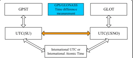
There is a system deviation between the time systems of different GNSS navigation systems, known as time dif-ferences. Taking the GPS/GLONASS time difference as an example, there is the following transformation be-tween GPST and GLOT:
GPST¼GLOTþτcþτuþτg ð17Þ
In this, τc represents the time difference between the
GLOT and the UTC (SU). τu represents the time
differ-ence between UTC (SU) and international UTC.τg
rep-resents the time difference between international UTC and GPST. The time difference between GPST and GLOT is the sum of the above three.
At present, the GPS’s broadcast ephemeris provides a linear time difference conversion model coefficient from GPST to UTC (USNO). The GLONASS broadcast ephemeris provides a time difference between GLOT and UTC (SU). Therefore, as long as the time compari-son between UTC (USNO) and UTC (SU) is obtained, the GPS/GLONASS time difference can be obtained.
The time comparison between UTC (USNO) and UTC (SU) can be obtained by direct comparison of the master stations or their comparison with international UTC or International Atomic Time (TAI). A brief process for obtaining a time difference through a time comparison technique at the end of the system is shown in the dia-gram in Fig.1.
The above time difference acquisition method has the advantages of high precision and stable and reliable time difference. It is one of the main ways to obtain the inter-national GNSS TDOA. However, this time difference ac-quisition method is usually performed on the main control station of the GNSS navigation system, and it needs to establish time comparison links between inter-national large time-frequency laboratories, and the oper-ation mode is not flexible enough. This also leads to the shortcomings such as poor real-time performance and the difficulty of direct acquisition by the user, which restricts its application in the actual navigation and positioning.
Based on this, this section will construct a feasible method for monitoring time difference directly in the cli-ent using a multi-mode receiver fusion PPP method. First, analyze the concept and nature of GNSS time difference required by the actual navigation and positioning user.
3.2 Concept of“pseudo-time difference”for navigation and positioning of users
For the navigation and location users of the multimode receiver, the most important contribution of the system time difference is to reduce the number of receiver clock parameters to be estimated, and then reduce the neces-sary satellite observations. Taking GPS/GLONASS as an
example, the receiver’s clock error parameter of GPS
system ^tGr and the receiver clock error parameter of GLONASS system ^tRr, absorb the absolute device delay
error b and inter-frequency relative equipment delay
errorδb on the respective system in addition to the real receiver clock difference tGr and tRr under its own time system. The specific formula expression is as follows [9]:
^tGr ¼tGr þbGþδbG ð18Þ
^tRr ¼tR
r þbRþδbR ð19Þ
Subtract the left and right sides of (18) and (19) by two and it could be obtained that:
^tsys¼^tGr−^trR¼tGr−tRr þ bG−bR
þδbG−δbR ð20Þ
The time difference ^tsys in the type (20) includes
both the real GPS/GLONASS system time difference tsysðtsys¼tGr−tRrÞ and the poor delay of the GPS/GLO-NASS device (bG−bR) + (δbG−δbR). The time
differ-ence of this property is called the “pseudo-time
difference” of the receiver.
It can be seen that the difference between the real time differencetsysand pseudo-time delay difference^tsys is the
equipment time delay (bG−bR) + (δbG−δbR) between GPS/GLONASS system. If the equipment time delay sig-nal of the GPS system and GLONASS system in the re-ceiver is the same, then the pseudo-time difference is real-time difference; otherwise, the two are not equivalent.
3.3 Acquisition of pseudo-time difference based on fusion PPP technology
First, the observational equations of the simplified fusion PPP are listed as follows:
PIF¼^ρþctrþbPþδbPþεð ÞPIF ð21Þ
ΦIF¼^ρþctrþbΦþδbΦþNþε Φð IFÞ ð22Þ
Among them, ^ρ represents the geometric distance
be-tween the station and the satellite after the correction of
the atmospheric error and so on. tr represents the
re-ceiver clock difference. The rere-ceiver’s code and phase device time delay is divided into two parts: one is the fixed time delay on the frequencybPandbφ, the other is the relative device time delay between the frequencyδbP andδbφ. For the phase observation, if the ambiguity par-ameter is a floating point solution, the fixed time delay bφ and relative time delay δbφ can be absorbed by the ambiguity parameter, and there is no need to solve in the actual navigation and location. For code observation, if the device delay is not corrected, it will be absorbed by the receiver clock error parameter, which will directly affect the absolute value of the receiver clock offset. Therefore, the absolute accuracy of the satellite clock difference is determined by the code observation value in the process of solving the actual satellite clock differ-ence. The phase observation value determines the rela-tive accuracy of the satellite clock difference calculation.
At present, IGS organizations provide three types of relative equipment delay correction products for code observations, also known as differential code deviation
correction products. It should be noted that in addition to DCB corrections for satellites announced in DCB products, DCB corrections on stations are also an-nounced. The measurement station DCB correction is often overlooked in GNSS positioning, mainly because it can be absorbed by the receiver clock skew and does not affect the actual navigation positioning solution. How-ever, in time difference monitoring, this correction is very important. It directly affects the magnitude of the receiver clock difference and must be subtracted from the observation equation.
DCB products with IGS can correct relative device
de-lays δbP between frequencies. However, absolute device
delay bP cannot be eliminated. In other words, the time
difference obtained by using the fusion PPP method is not a true time difference, but a pseudo-time difference con-taining the poor delay of the absolute equipment between systems, which can be expressed by the following formula:
tsys¼tsysþ bGP−bRP
ð23Þ
It can be seen from the above equation that when the absolute device delays of different navigation systems are the same, the fusion PPP gets the real system time differ-ence sequdiffer-ence. In fact, the absolute device delays of dif-ferent navigation systems in the same receiver are different, and the phase difference can range from a few nanoseconds to hundreds of nanoseconds.
4 Experience
In order to compare and verify the efficiency and accur-acy of this algorithm, the following two types of exam-ples are designed to verify it.
4.1 Comparison of operational efficiency
First, 1000 epoch observation data for the four naviga-tion systems GPS, GLONASS, COMPASS, and Galileo were simulated. Each system has ten observation satel-lites per epoch. Satellite replacement does not occur during the observation period. The computational effi-ciency of multi-mode fusion PPP positioning based on traditional algorithm and parameter reduction is calcu-lated respectively. Fusion static PPP location calculation of single-system, dual-system, three-system, and four-system is performed. The data processing carrier is based on a high-performance configuration computing computer. Both schemes use different numbers of GNSS systems for fusion PPP positioning. The computational time statistics needed to process 1000 epochs are shown in Fig.3:
As can be seen from Fig. 2, with the increase in the
shows a linear increase in processing time. With the wide application of multi-mode systems, the computational ef-ficiency of this algorithm is significantly higher than the traditional algorithm.
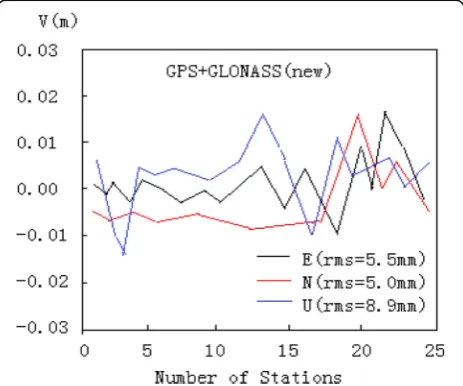
4.2 Static and dynamic accuracy test of fusion positioning In order to further verify the correctness of the fusion PPP location algorithm and the effectiveness of the adap-tive factor, the measured GPS/GLONASS dual-system ob-servation data is used for calculation and analysis. The data comes from the global IGS tracking and monitoring network, and 24 IGS stations equipped with GPS/GLO-NASS dual-mode receivers that are evenly distributed on the European continental plate are selected for static PPP calculation. The data sampling rate is 30 s. The total ob-servation period of data is 24 h.
Two scenarios were designed for comparative analysis: case 1, fusion PPP positioning based on parameter reduc-tion, and case 2, self-adaptive fusion PPP positioning based on the posttest difference. Using the coordinates of the stations posted on the IGS website as “true values,” the deviation values of the positioning results of each sta-tion in N, E, and U directions were calculated, and the overall RMS indicators corresponding to the deviation values of all stations were calculated. The statistics of devi-ations and RMS values of static PPP positioning results for specific experiments are shown in Fig.3.
It can be seen from Fig. 4 that for a single-day solu-tion, in the dual system fusion PPP positioning, the posi-tioning accuracy on the plane can reach the millimeter level. The accuracy of the elevation direction is also maintained at about 1 cm. This aspect shows good ob-servation conditions at the IGS tracking station. On the other hand, it also illustrates the high-precision features of current PPP technology. Scenario 1 uses only equal
weights to carry out the normal equation stacking and cannot reasonably assign the weight ratio relationship between GPS and GLONASS observations. The resulting fusion location results and accuracy lie between the po-sitioning accuracy of the two single systems. The use of a posterior misalignment for adaptive fusion positioning (case 4) solves this problem better and has the best posi-tioning accuracy.
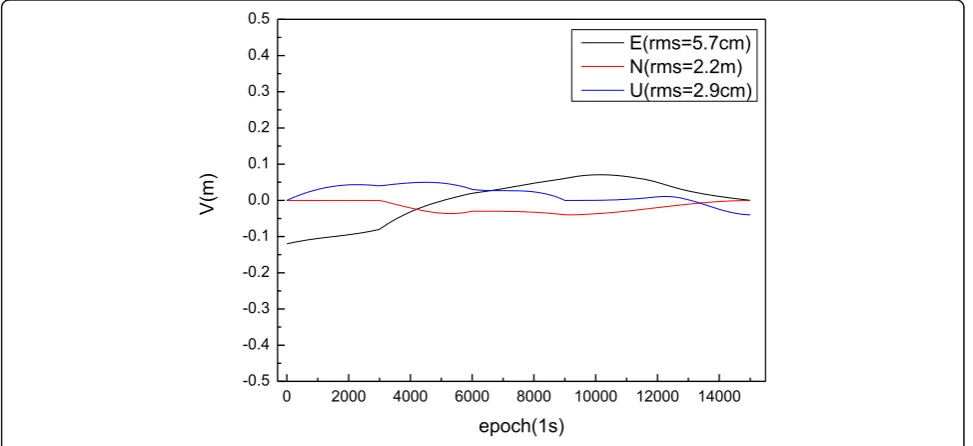
In addition, in order to further verify the effectiveness and accuracy of the proposed algorithm in dynamic PPP lo-cation, a high-frequency IGS monitoring station equipped with a GPS/GLONASS dual-mode receiver was selected for dynamic PPP calculation. The data sampling rate is 1 s, and the total data observation duration is 5 h. Using the coordi-nates of the stations published on the IGS website as the “true value,”the sequence of deviations in theN,E, andU Fig. 2Time information of multi-system fusion PPP processing
carried out by two methods Fig. 3Positioning result deviation and RMS value of case 1
directions of the station’s dynamic positioning results was calculated and the corresponding RMS values were calcu-lated. The statistics of the dynamic PPP positioning devi-ation sequence and the RMS index value for specific experiments are shown in Fig.5.
It can be seen from Fig.6 that whether it is equal-value fusion PPP (case 1) or adaptive fusion PPP (case 2), the dy-namic positioning accuracy is better than the single-system PPP positioning result. This shows that multi-system fusion positioning has significant advantages for improving the accuracy of dynamic positioning. When the observation
conditions are good, the positioning accuracy of the two conditions is basically the same.
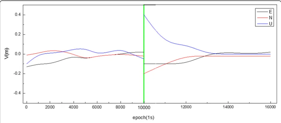
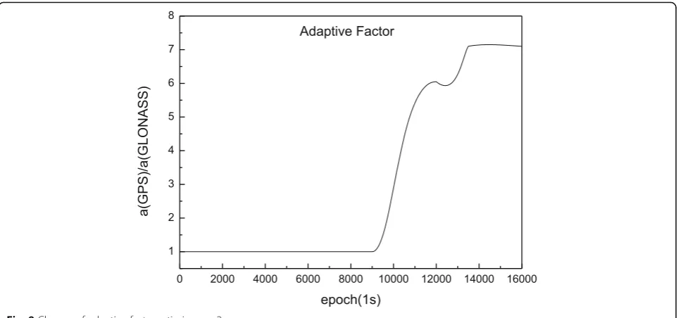
In order to further analyze the validity of case 2 in the presence of gross errors in observations, this article adds a phase error of 1 m to the first GPS satellite of each epoch during the 10,000th to 12,000th epoch of dynamic stations. The observations after 10,000 epochs were compared using case 1 and case 2. The positioning re-sults are shown in Fig.7.
The change in the ratio of the adaptive factor of GLO-NASS to GPS of case 2 is shown in the following diagram. Fig. 5Dynamic positioning deviation and RMS value of case 1
From Figs.7,8, and9, it can be seen that when there is a rough difference between the observed values of a single system, the location results of case 1 are ser-iously affected, and the situation 2 is less affected. The reason is that when a single system experiences a gross error in observations, the resulting single-system test posterior error will gradually become larger, so that the adaptive factor of case 2 will be automatically adjusted to redistribute the fusion weight ratio rela-tionship of different systems and reduce the gross error ratio and reduce the contribution of system nor-mal equations with gross errors to achieve the purpose of suppressing gross errors.
4.3 Short term stability of fusion PPP pseudo-time difference results
In this section, the data of 14 GPS/GLONASS observa-tion staobserva-tions in the IGS continuous tracking staobserva-tion net-work in the European region were uniformly selected for analysis [10]. The data acquisition time is March 22, 2012, the data sampling rate is 30 s, and the total obser-vation time is 24 h. The satellite orbit and clock differ-ence products are derived from the IAG products provided by the MCC Analysis Center under the IGS organization. The GPS/GLONASS orbit of IAG products has been classified into the ITRF framework, and the satellite clock difference is kept under the respective Fig. 7Dynamic positioning deviation and RMS value of case 1 (with gross error)
time system. The sampling rate of the track product is 15 min, and the sampling rate of the clock difference product is 5 min. All stations are equipped with dual fre-quency dual mode GNSS receivers. In order to compare the difference in the result of the time difference be-tween the different receiver types, the station name and the receiver type information are listed, as shown in Table1:
As you can see from Table1, there are six kinds of re-ceiver types in the 13 selected stations. There are six sta-tions in which the LEICA receiver is equipped. Four stations are equipped with TRIMBLE receivers. The other types of receivers have only one station configur-ation each. The mean and standard deviconfigur-ation of the time difference sequence on all stations are counted, as shown in the Table2:
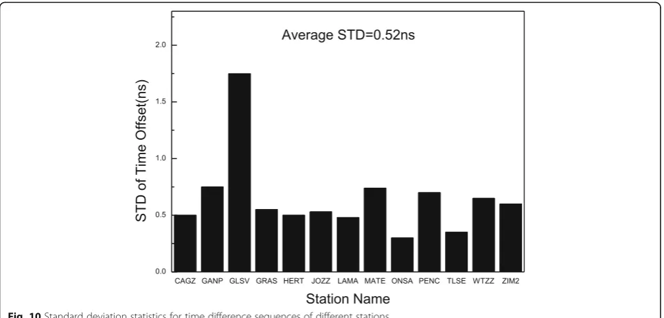
The standard deviation index of the time difference sequence of different stations is compared, as shown in Fig.10.
The Allen variance is used to calculate the single day frequency stability index of time difference sequences of the different station, such as 11.
As can be seen from the graph in Figs.10and11, the
result of the time difference sequence obtained by the same type of receiver is relatively close, and the absolute difference of the time difference is less than 20 ns. This is mainly due to the close proximity of the absolute hardware delay of the same type of receiver, so the time difference sequence is relatively close. There is a large system error due to the difference of absolute hardware delay between different receivers[11]. The maximum Fig. 9Change of adaptive factor ratio in case 2
Table 1Station name and the receiver type information
Station name Receiver type Station name Receiver type
CAGZ TPS E_GGD PENC LEICA CR × 1200
ONSA JPS E_GGD GANP TRIMBLE NETR8
GLSV NOV OEMV3 GRAS TRIMBLE NETR5
HERT LEICA CR × 1200 TLSE TRIMBLE NETR9
JOZ2 LEICA CR × 1200 ZIM2 TRIMBLE NETR5
LAMA LEICA CR × 1200 WTZZ JAVAD TRE_G3TH
MATE LEICA CR × 1200
Table 2Mean and standard deviation of the time difference sequence (unit: nanosecond)
Station name Receiver type Mean Standard deviation
CAGZ TPS E_GGD −448.257 0.423
ONSA JPS E_GGD −464.486 0.286
GLSV NOV OEMV3 −348.679 1.123
HERT LEICA CR × 1200 −337.857 0.546
JOZ2 LEICA CR × 1200 −353.536 0.475
LAMA LEICA CR × 1200 −345.758 0.389
MATE LEICA CR × 1200 −333.689 0.732
PENC LEICA CR × 1200 −345.785 0.598
GANP TRIMBLE NETR8 −374.537 0.694
GRAS TRIMBLE NETR5 −375.974 0.645
TLSE TRIMBLE NETR9 −364.876 0.432
ZIM2 TRIMBLE NETR5 −384.438 0.564
mean time difference is more than 130 ns. The result of the time difference sequence on all stations is very stable in 1 day. Most of the standard deviation of the time dif-ference sequence is better than 1 ns, and the average standard deviation is only 0.52 ns. This stable character-istic provides a good premise for the follow-up time dif-ference prediction and the application in navigation and positioning[12]. The single-day frequency stability ana-lysis of the TDOA sequence shows that the single day stability index of the TDOA sequence obtained by the
fusion PPP is about the magnitude of 10−14, and the
average frequency stability is 3.0 × 10⁻¹⁴. This shows that it is feasible to use the fusion PPP method to monitor the time difference of the system from the precision[13].
5 Results and discussion
The traditional multi-mode GNSS fusion precise single-point positioning algorithm has the disadvantages of low efficiency and difficulty in satisfying the demand for high-accuracy real-time and high-frequency data[14]. To solve the above problems, this paper proposes an adap-tive GNSS fusion PPP algorithm based on parameter Fig. 10Standard deviation statistics for time difference sequences of different stations
equivalence reduction. With the increase of the number of fusion systems, the computing load of traditional al-gorithms is exponentially increasing. The new algorithm improves it to a linear growth, which greatly improves the computational efficiency. The actual example verifies the effectiveness and accuracy of the improved algo-rithm. Secondly, this paper also studies the feasibility and algorithm flow of GNSS time difference monitoring using multi-system fusion PPP algorithm at the user end. Pseudo-time difference monitoring and forecasting work has more important application value for naviga-tion and posinaviga-tioning users[15]. The real system time dif-ference has no practical significance for navigation users.
Abbreviations
GLONASS:GLObalnaya NAvigatsionnaya Sputnikovaya Sistema; GNSS: Global Navigation Satellite System; GPS: Global Position System; PPP: Point-to-Point Protocol; UTC: United Technology Corporation
Funding
Technology Platform Project of Guangdong Provincial Department of Education (2017GKTSCX104), Plan Project of Guangdong Science and Technology (2014A010103002)
Availability of data and materials
The datasets used and/or analysed during the current study are available from the corresponding author on reasonable request.
Authors’contributions
ZZ carried out the time difference detection algorithm studies, participated in the sequence alignment and drafted the manuscript. ZX and HC carried out the Data test. JY and YL participated in the sequence alignment. WZ participated in the design of the study and performed the statistical analysis. YC conceived of the study and participated in its design and coordination. All authors read and approved the final manuscript.
Authors’information
Ziwen Zhang, Male, Postdoctoral, 1987-11-25, Guangdong University of Technology.
Major: High-precision satellite positioning, radar interferometry, deep learning.
Jun Yang, Male, postgraduate, Chongqing Vocational College of Transportation.
Main research direction: high-precision satellite positioning, radar interferometry, deep learning.
Yijun Liu, Male, Professor, Guangdong University of Technology. Major: High-precision satellite positioning, deep learning.
Zuoteng Xu, Male, Master student, Guangdong University of Technology, Communication Engineering.
Main research direction: Deep learning, computer graphics processing. Haowen Chen, Male, Master student, Guangdong University of Technology. Main research direction: Deep learning, computer graphics processing. Yuqiang Chen, Male, Professor, 1983-07-13, Gongguan Polytechnic. Main research direction: Satellite high-precision positioning, artificial intelligence.
Competing interests
The authors declare that they have no competing interests.
Publisher’s Note
Springer Nature remains neutral with regard to jurisdictional claims in published maps and institutional affiliations.
Author details
1Chongqing Vocational College of Transportation, Chongqing 402247, China. 2School of Information Engineering, Guangdong University of Technology,
Guangzhou 510006, China.3Dongguan Polytechnic, Dongguan 523000,
China.
Received: 29 December 2018 Accepted: 26 March 2019
References
1. Z. Hongping, Z. Gao, X. Niu, et al.,Research on GPS precise point positioning with un-differential and un-combined observationsGeomatics & Information Science of Wuhan University28(6), 217-221 (2013)
2. W. Jiang, Y. Li, C. Rizos,An optimal data fusion algorithm based on the triple integration of PPP-GNSS, INS and terrestrial ranging system(2015)
3. Q. Zhao, B. Sun, Z. Dai, et al., Real-time detection and repair of cycle slips in triple-frequency GNSS measurements. GPS Solutions19(3), 381–391 (2015) 4. H. Zhang, Z. Gao, M. Ge, et al., On the convergence of ionospheric
constrained precise point positioning (IC-PPP) based on undifferential uncombined raw GNSS observations. Sensors13(11), 15708–15725 (2013) 5. Q. Zhang, S. Tan, S. Yang, GNSS system time bias estimation based on PPP.
J. Geom.41(01), 27-30 (2016)
6. C. Liang, H.U. Zhigang, C. Geng, et al., Study on a high-frequency multi-GNSS real-time precise clock estimation algorithm and application in multi-GNSS augment system. Acta Geodaetica Et Cartographica Sinica.45(S2), 12-21 (2016)
7. M. Ge, G. Gendt, M. Rothacher, et al., Resolution of GPS carrier-phase ambiguities in precise point positioning (PPP) with daily observations. J. Geod.82(7), 389–399 (2007)
8. M.R. Kaloop, M. Rabah, Time and frequency domains response analyses of
April 2015 Greece’s earthquake in the Nile Delta based on GNSS-PPP. Arab. J. Geosci.9(4), 1–13 (2016)
9. Tobías G, Calle J D, Navarro P, et al. magicGNSS’Real-Time POD and PPP Multi-GNSS Service. 2014
10. G. Huang, Y. Yang, C. Liu, et al., GNSS precise point positioning algorithm based on parameter equivalent reduction principle. Lect. Notes. Elect. Eng.
244, 449–469 (2013)
11. N. Noomwongs, R. Thitipatanapong, S. Chantranuwathana, et al., Driver behavior detection based on multi-GNSS precise point positioning technology. Appl. Mech. Mater619, 327–331 (2014)
12. G. Huang, Q. Zhang, Real-time estimation of satellite clock offset using adaptively robust Kalman filter with classified adaptive factors. GPS Solution (2012).https://doi.org/10.1007/s10291-012-0254-z
13. N. Abdi, A.A. Ardalan, R. Karimi, et al., Performance assessment of multi-GNSS real-time PPP over Iran. Adv. Space Res.59(12), 117-123 (2017) 14. U. Weinbach, S. Schön, GNSS receiver clock modeling when using
high-precision oscillators and its impact on PPP. Adv. Space Res.47(2), 229–238 (2011)