Earth Planets Space,56, 217–227, 2004
Genetic Algorithm inversion of geomagnetic vector data using a 2.5-dimensional
magnetic structure model
Michiko Yamamoto1, and Nobukazu Seama2
1GEOMAR Forschungszentrum fur marine Geowissenschaften, Wischhofstrasse 1-3, D-24148 Kiel, Germany 2Research Center for Inland Seas, Kobe University, 1-1 Rokkodai, Nada, Kobe 657-8501, Japan
(Received June 25, 2003; Revised December 18, 2003; Accepted January 23, 2004)
We propose a new inversion method for vector magnetic field data, which uses the Genetic Algorithm in a space domain calculation to determine the best-fitting 2.5-dimensional (2.5-D) structure. This 2.5-D model is composed of magnetic boundaries with arbitrary strike and magnetic intensity. Two numerical formulas combine to express this model. One of them is a two-dimensional magnetic structure expression for a realistically shaped magnetic layer, and the other is a magnetization contrast expression for magnetic boundaries of variable strike. We use a Genetic Algorithm as the computational technique that supports optimum solutions for magnetization, magnetic strike, and boundary location. In practice, calculations are more accurate in the space domain instead of the more conventional frequency domain because it better preserves the short wavelength components and the true geometry between magnetic sources and observation points even for uneven survey track lines. The above leads to high resolution in the inferred magnetization without the need of upward continuation, which is particularly useful for inverting near-bottom survey data. The code is designed to use smaller storage and less computational time. Its application to synthetic data illustrates the power of resolution and precision in interpreting the fine scale processes of mid-ocean ridge accretion.
Key words:Genetic Algorithm, geomagnetic vector data, near-bottom survey, 2.5 D magnetic structure.
1.
Introduction
A key discovery leading to plate tectonics was the obser-vation that the Earth’s magnetic field reversals are preserved during the formation of the ocean crust, thereby creating lin-eated magnetic anomaly stripes (Vine and Matthews, 1963; Morley and Larochelle, 1964). Magnetic surveys are com-monly conducted over all the ocean basins, although many recent studies have focused on studying detailed phenomena of seafloor accretion. This new focus demands both higher resolution data and high-resolution analysis methods. The most significant improvements in data collection have come from conducting near-bottom surveys and collecting vector magnetic data. Although there remain difficulties in its ac-curate measurement, which is affected, for instance, by unex-pected sensor motion, vector data provide much more useful magnetic information in comparison with total field-intensity measurements.
The use of vector magnetic data was pioneered by Isezaki (1986) who showed the degree of two-dimensionality in the magnetic layer by means of the phase shift between the hor-izontal and vertical components along the profile. He also proposed a method to detect the strike of the magnetic lin-eation by determining the direction in which the amplitude of horizontal compornent is minimal. It is a useful technique to estimate structural directions from surface data, but is less useful for interpreting near-bottom survey data becasue it
Copy right cThe Society of Geomagnetism and Earth, Planetary and Space Sciences (SGEPSS); The Seismological Society of Japan; The Volcanological Society of Japan; The Geodetic Society of Japan; The Japanese Society for Planetary Sciences; TERRA-PUB.
is designed to detect one direction for one survey line, and near-bottom surveys detect finer-scale information that needs to be preserved. The intensity of spatial differential
vec-tors (ISDV) method proposed in Seamaet al.(1993) made
it possible to search for various orientations of the magnetic boundaries along a single survey track line. They also men-tioned that ISDV has a weakness in the low spatial resolution of its boundary detection, which is limited to one-and-a-half times the water depth.
Most existing methods for calculating magnetization are FFT (Fast Fourier Transform)-based algorithm developed by
Parker (1972), Parker and Huestis (1974), and Macdonaldet
al.(1980). These method are computationally effective and
become a standard routine. On the other hand, this method and other FFT-based methods have the inconvenience when dealing with near-bottom survey data where the survey track should always be treated at a constant depth. The upward continuation of observed anomalies onto a synthetic even al-titude results in the loss of finer-scale information, thus los-ing most of the advantage of painstaklos-ing near-bottom
sur-veys. Hussenoederet al.(1995) propose a method to save
short wavelength information. In their method, the track depth is approximated as a constant level, and the seafloor relief is corrected using the real distance between the sen-sor and seafloor bottom. This method can retain short wave-length signals and mathematically compensate the artificial change of direct distance between a magnetic source and lat-eral observation points.
The previous methods are generally based on the assump-tion of a two-dimensional (2-D) magnetic structure and none
y
1
y
5
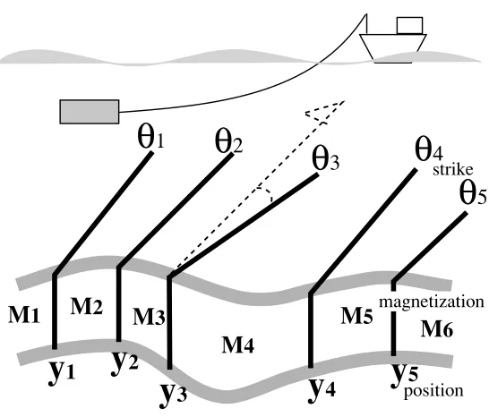
Fig. 1. The 2.5-D magnetic structure. Vertical planes that have variable strike represent magnetic boundaries. Various strikes are indispensable to express changes of the spreading direction on the mid-ocean ridge and to know true magnetization influenced by unexpected magnetic boundaries like lava flows or tectonic lineations like fault throws. This study searches for the unknown parameters magnetization (M), magnetic boundary’s strike (θ), and position (y).
of them determines the seafloor magnetization and magnetic boundary at the same time. Because the magnetic struc-ture that we look for varies in both magnetization and mag-netic boundaries that are inter-related, simultaneous solution would be better.
The proposed method in this paper is motivated by the de-mands for the analysis of near-bottom vector magnetic sur-veys and/or surface vector magnetic sursur-veys, with the goal of taking full advantage of the information contained in the vector data. To satisfy this goal, the method must meet three challenges. First, it must cope with the effects of a short dis-tance to a non-2D magnetic source, topography variations, and uneven survey tracks. Second, its numerical resolution must not degrade the near-bottom observations. Third, it should have the convenience of simultaneously calculating all of the important parameters in a magnetic structure with-out requiring an accurate initial model to convergence with a good global solution.
In this study, we propose a method for analyzing vec-tor magnetic data that uses a more realistic 2.5-dimensional (2.5-D) magnetic modeling technique within a Genetic Al-gorithm (GA) inversion. To present this method, we will in-troduce the 2.5-D structure model which can include detailed magnetic layer information. Then, we will describe the code design using the GA and its subsidiary iterative improvement method. After presenting the method, we will show an appli-cation to synthetic deep-tow vector magnetic data to examine its benefits and the reliable solutions found for uneven survey tracks.
2.
2.5-Dimensional Model of Magnetic Structure
We use the 2.5-D magnetic structure model shown in Fig. 1. Its distinctive features are the incorporation of
vari-ous strikes of magnetic boundaries and a detailed expression of the magnetic source layer. Various strikes are expressed by vertical planes, and the magnetization distribution (ver-tically homogeneous) includes intensity changes within the same polarity interval to cope with dipole field fluctuations. The expression of variable boundary strikes is especially im-portant for near-bottom surveys to determine the magnetiza-tion because near bottom data are sensitive to near-surface magnetic structures like lava flow boundaries. The assump-tion of a variable angle strike enables the determinaassump-tion of the magnetization without adverse influence by the assump-tion of parallel boundaries. Addiassump-tionally, the assumpassump-tion of a variable strike lets the data reflect the structural complexity of the seafloor at a local scale. A detailed expression for the magnetic layer is achieved by 2-D magnetic blocks of an ar-bitrary trapezoid section. Two parallel lines are used for the vertical magnetic boundaries; the upper and lower bound-aries can follow the shape of the upper and lower boundbound-aries of the magnetic layer.
The 2-D block model expression is based on that of Blakely (1995), originally used for an infinite extent hori-zontal ribbon.
where X and Y coordinates are perpendicular and parallel to survey track respectively, and the Z coordinate is vertical. M
is magnetization,ˆs andn are unit vectors parallel and normalˆ
to the ribbon, r1 and r2 are distance from the observation
point to the two edges of the ribbon, andθ1 andθ2 are the
M. YAMAMOTOet al.: GA INVERSION USING A 2.5-D MAGNETIC STRUCTURE 219
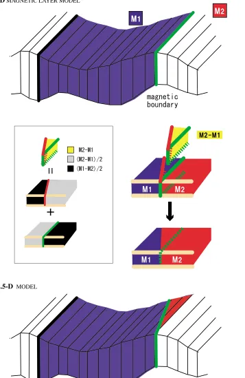
Fig. 2. Illustration for the mechanism to change a boundary strike. Each color shows a different magnetic intensity. Blue has magnetization M1, red has magnetization M2, yellow, gray and black have M2-M1, (M2-M1)/2 and (M1-M2)/2 respectively. a) Combinations of 2-D blocks with a polygonal cross-section (trapezoidal section in this study) describe the detailed magnetic layer structure. (middle left box) Two magnetic structures, one with the original strike parallel to the 2-D model (lower block model with green strike) and the other with the predicted strike (upper model with red strike), are superimposed to add their magnetization to make a wedge-shaped magnetic body (yellow in top). (middle right). Boundaries can smoothly change their strikes to another direction by embedding the wedge body along the original 2-D block boundary. b) 2.5-D model with an arbitrary strike after the above steps.
made a block model with parallel boundaries assuming the parallel direction is fixed to the X axis. These equations are used for the detailed expression of the magnetic layer shape and its intensity distribution (Fig. 2(a)). Such a 2-D block
model has fixed boundaries parallel to the strike, therefore we need another expression to change strikes which is given below.
mag-netic boundary in a horizontal magmag-netic layer of infinite ex-tent. Vacquier’s (1972) result is slightly rearranged for the magnetic field by magnetization contrast;
J=J(Jˆx,Jˆy,Jˆz),
nent) and a uniform vector direction is assumed. h1andh2
are the depths of the upper and lower boundaries of the
mag-netic layer, y−y0 is the horizontal distance between
obser-vation points and the magnetic boundary, andθ andα
rep-resent the azimuths of the boundary and survey track. Fig-ure 2 illustrates our idea to express the changing strike of a boundary. Here, two magnetic structures each consist of a magnetic boundary between two adjacent magnetic blocks. The differences between the two structures lie in the bound-ary’s strike and magnetic polarity. In the one structure, the strike is parallel to the direction fixed by 2-D blocks, in the other it may vary (Fig. 2(a)). The two blocks are also oppo-sitely placed, resulting in an opposite polarity contrast. First, these two structures are superimposed and their magnetiza-tion added to make a wedge-shaped magnetic body. Next, the wedge body is embedded along the original 2-D block boundary, and then the boundaries smoothly change their strikes to another direction (Fig. 2(b)). One of the merits derived from deliberately taking another step for changing strikes is to avoid boundaries that cross each other just on a track.
Both equations operate in the same coordinate system. The configuration of the observational point and magnetic
source determine the choice of y0,h1,h2,r1,r2, θ1 and θ2.
When the given parameters are azimuth of survey lines, magnetization direction, and magnetic layer shape, there are
three different types of unknown parameters, θ , y and M.
J is automatically determined by M, because M defines J as Ji =Mi+1−Mi.
3.
Computational Techniques
For the basic inversion, we used a Genetic Algorithm (GA) (Goldberg, 1989). The GA is an evolutionary com-puting algorithm which is inspired by Darwin’s theory about evolution. A great advantage of GA is in its parallelism. Af-ter the code initializes a random sample of many individu-als with different parameters, the GA operator travels in a search space with gradually evolving individuals to be opti-mized until a user-specified level of convergence is achieved.
As mutations sometimes happen, this strategy is less likely to get stuck in local convergence than some other iterative inversion methods. If the mainstream goes to local conver-gence, at the same time the operator keeps searching other regions of the solution space by random mutations.
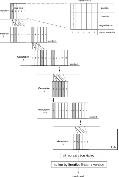
The GA program is implemented in the following cycle. To begin with, we specify the minimum and maximum val-ues of parameters to set the search range and specify the number of model-defining bits that directly relate to the res-olution of the GA search. The use of more bits permits a higher resolution solution at the expense of a longer compu-tation time. The GA operator starts encoding ‘chromosomes’ that are binary strings of combination ‘0’ and ‘1’ gathered randomly along the model-spaces bit number. All chromo-somes together make a set called the model ‘population’. After decoding the population, each chromosome is given a ‘fitness score’ that depends on how ‘good’ each chromo-some is (for example, in this paper, fitness is defined as the standard deviation (SD) between the observed magnetic pro-file and calculated forward solution propro-file). Next, parents are selected according to their fitness. The ‘better’ a chro-mosome fits the observation, the more chances of being se-lected. Then, crossover and mutation steps are performed on the re-coded population. The crossover routine selects two parent chromosomes from the population and mixes a part of their genes (bits) to create a new offspring chromosome, and this is repeated until a full list of new offspring is built. The mutation step may randomly change the new offspring by switching a few randomly chosen bits from 1 to 0 or from 0 to 1. This is to prevent all solutions in the population from falling into the same local minimum. Finally, the offspring population replaces their parent population. In this paper, we modify this strategy in the so-called ‘micro-GA’ approach. This process runs as described above except for the mutation section. Mutation never occurs in this micro-GA, but only crossover between chromosomes, which continues until the 90% of the population is identical. This “evolution without mutation” has resulted in strong heredity traits of the best-scoring previous generation. Next, chromosomes in the pop-ulation are all discarded except for this top score, and the rest of the population is again randomly initialized. The infor-mation in this GA scheme evolves more slowly than in some alternatives, but with a higher chance to search a wider range of the solution space than by ’normal’ mutation schemes. For this problem, we have found that the micro-GA finds better solutions in less computation time than standard GA algo-rithms do.
con-M. YAMAMOTOet al.: GA INVERSION USING A 2.5-D MAGNETIC STRUCTURE 221
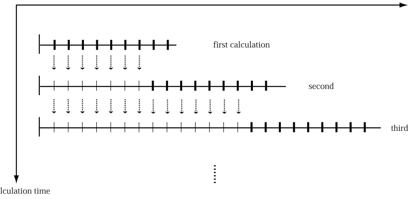
Fig. 3. Progressive search range along a survey track line. Thick bars represent unknown magnetic boundaries as search parameters in each GA calculation. Thin bars are results from the calculation for a previous subregion. The GA algorithm determinate parameters to fit the observed profile with the forward profiles calculated from a combination of both new parameters and previous parameters. Note some boundaries near the end of the calculation range are discarded in the next calculation because of their lower reliability (since they do not yet include information from the next subregion).
trast.
For a faster and more memory efficient algorithm, each inverse GA calculation solves for sequential subregions (Fig. 3), including information from each previous subregion as it becomes available. This results in more realistic solu-tions that contain comprehensive information from the whole profile.
The biggest limitation to the GA algorithm is the discrete limits for internal boundary segments. In many cases, the GA algorithm smoothly moves to a near-optimal solution. However, the GA algorithm is not the best way to find a better ‘refined’ solution because of its inefficient approach to slightly changing its parameters and so ‘polish’ its best approximation solution. For example, in this algorithm the search range does not adjust in the middle of a GA calcu-lation to a narrow region around a candidate ‘optimal solu-tion’. Another problem is the discrete possible steps for in-ternal boundary locations and other model parameters. It’s easy for the GA operator to select one when either of the serrated teeth is near-optimal. However, what if the ‘opti-mal’ solution parameters lie between the GA’s discrete pa-rameter choices? In this case, the GA naturally takes the next best parameters. However, several computational ex-periments show that second best, as defined by the degree of fitness, is not always visually closer to the right solution, and will depend on the discretization interval. For example, when the GA algorithm tries to make a big magnetic contrast in an ‘impossible position’, it will usually create two small magnetization steps on both sides of the ‘best’ position, in-stead of a single, bigger contrast at the would-be center. This trait leads to a wrong direction of convergence unless the so-lution teeth happen to be disposed correctly. However, con-ventional inversion methods using iteration techniques with differential coefficients can easily ‘improve’ this GA weak-ness in finding a ‘best’ local minimum—their problem is that they do not search a broad parameter range as do the GA
methods before ‘converging’ onto a particular local minima. Hence, using GA as the primary search tool, followed by use of a standard iterative inversion routine as a secondary solution—‘polishing’ tool is an effective way to combine the complementary strengths and weaknesses of the two inverse approaches.
However, one problem arises when the GA algorithm de-livers the solution parameters to the following inversion step. The GA solution often includes extra boundaries which will be improper initial settings for the standard inversion tech-nique. These create too small magnetic contrasts or too nar-row boundary intervals that bring less effect to a forward pro-file, otherwise they are substitutes for an optimal solution be-tween the GA’s parameter choices. We have found that omit-ting those extra boundaries leads to better results than some restraint conditions included in GA implementation that al-ways result in bad fitness chromosomes. Therefore, we insert an additional step to omit the extra boundaries when switch-ing from the GA to the linear inversion polishswitch-ing step.
Consequently, our detailed ‘recipe’ for the inverse prob-lem is the following. Firstly, use the usual GA algorithm, secondly omit the extra boundaries just before the GA cal-culation is terminated, finally polish the ‘best’ GA solution with a standard linear-inversion scheme (Fig. 4).
M. YAMAMOTOet al.: GA INVERSION USING A 2.5-D MAGNETIC STRUCTURE 223
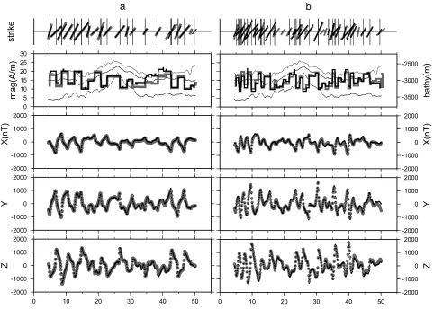
Fig. 5. Comparison between normal GA search solutions and true solutions; forward model search solutions and model parameters. (a) Larger interval, (b) smaller interval of boundaries. (top) Boundary strike on each solution at detected boundary position. The thin vertical bar represents north-south direction. The bold, gray bar and black thin bar show the true boundary azimuth and search boundary azimuth respectively. The length of the bar is in proportion to the magnetic contrast. (second from the top) Relative variations of magnetization with left scale. Bathymetry, magnetic layer bottom profile given by seismic experiment and fish track with right scale. The bold gray line and thin black line show the true and search magnetizations parallel to the dipole direction. (upper, lower, bottom) Comparison between each component of the anomaly field (bold light line) and the forward model calculation (black dots). X, Y and Z components represent along and perpendicular to track directions and the vertical, respectively.
extract better, more realistic solutions.
4.
Application and Results
We now demonstrate, step by step, how our method works in practice for a synthetic magnetic profile. We also show results when applied to a profile in a longer wavelength than the width of each calculation window in order to verify that solutions can properly handle exterior magnetic effects out-side of the solution window. In this demonstration, we as-sume the ‘observed’ profile to be a forward model calculated from an arbitrary magnetic intensity variation with real to-pography and magnetometer depths from a vector magnetic
deep-tow survey over the Southern East Pacific Rise (18◦S)
during MOAI (Mid-Ocean ridge Axial Investigation and
In-strumentation) 1998 cruise (Seamaet al., 1997; Yamamoto
et al., 1998). The layer 2A pattern of the forward magnetic
source layer is based upon seismic results (Carbotte et al.,
1997). An uneven survey track is chosen to lie roughly 200 m above the seafloor.
The result of using only normal GA methods is shown in Fig. 5. A 50 km-long profile is divided into 16 windows. The conditions during the GA inversion of each window are the following: 300 generations, 9 search boundaries with 0.5
km interval corresponding to a 4.5 km discretization and 45
((3+2)×9) search parameters ((magnetization, position and
strike parameters+2 sign parameter for strike and position)
×9 search boundaries), 126 bits per chromosome (4 bits
for 3 magnetic parameters and 1 bit for 2 sign parameters), 126 candidates in the test population, search ranges of
mag-netization, position and strike are 6–22 A/M,±245 m from
the basic reference at 500 m intervals, and±20◦ from 30◦,
respectively. These conditions correspond to candidate
solu-tion resolusolu-tions of 16 m, 1.06 A/M, and 1.3◦. The GA search
Z
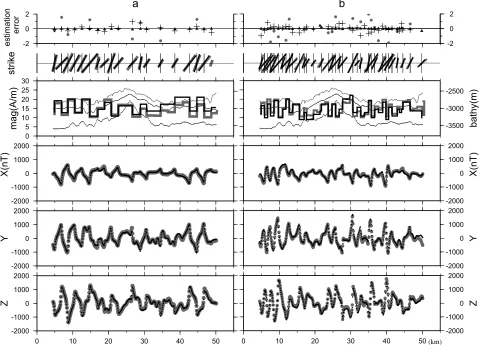
Fig. 6. Comparison between a normal GA search followed by excess boundaries omission and true solutions. (top) Estimation error. Cross shows magnetization (A/m), circle for magnetic boundary strike (degree) and triangle for boundary position (km). See explanation for other signs in Fig. 5.
steps. This especially happens if a better solution lies in an opening between the discrete choices available for the GA algorithm, as mentioned above. Figure 5(b) shows the result from using a model observation profile with short interval boundaries. The very small SD value (30–50 nT) compared
to the amplitude of the observed profile (2000 nT)
sug-gests a good convergence for each of the profiles (SD values of X, Y and Z are 30, 48 and 47 nT, respectively). Extra boundaries like the long interval case of Fig. 5(a) are rather subdued here, although some extra boundaries still survive. Larger contrast boundaries are well-fit in all kinds of param-eters, but smaller contrasts almost fail in their inferred strike. It is difficult for GA operator to find inconspicuous small boundaries because these boundaries make quite small con-tributions to the magnetic anomaly. The strike contribution is especially obscure. In addition, empirically the conver-gence rate rapidly drops after reaching a converconver-gence level like those shown in Figs. 5(a) and (b).
Figure 6 shows the situation after automatically thinning out boundaries. (300 generations set for usual GA and 100 generation for coordinating boundary number; 1.06 A/M change compared with its neighbors or narrower than 0.3 km blocks are omitted.) This clearly improves the magnetization estimates in longer, flat areas. Now, the number of internal boundaries is near the true number, while the fit between ‘ob-served’ and calculated profiles is slightly worse (SD values
of X, Y and Z are 29, 28 and 38 nT in Fig. 6(a), and 40, 61 and 57 nT in Fig. 6(b)) compared to the fit before removing the fine peaks. The estimated error is also shown on the top box in Fig. 6. These plots indicate a relatively bigger disper-sion in the ‘best-fit’ strike, with better convergence for the internal boundary position and magnetization.
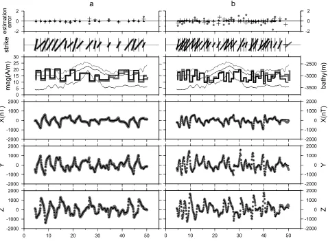
Figure 7 shows the final solutions after an iterative linear-inversion improvement step (100 iterations, with dumping factors of 0.1 for strike and 0.01 for other parameters). The resulting inverse solutions almost recover the initial forward model parameters except for a few secondary boundaries. The fit is also improved (SD values of X, Y and Z are 9, 12 and 12 nT in Fig. 7(a), 19, 29 and 28 nT in Fig. 7(b)). The iterative improvement step is primarily tuned to act on the strike parameter rather than the position and magnetization parameters that the GA has already well-located. In general, we suggest choosing dumping factors to allow large changes in the strike parameters and just minor adjustments to the other parameters, because allowing full variation simultane-ously under imperfect boundary conditions can easily cause the iterative scheme to diverge. In practice, setting the dump-ing factors in this way leads the solution to swiftly settle into a stable improved minimum.
M. YAMAMOTOet al.: GA INVERSION USING A 2.5-D MAGNETIC STRUCTURE 225
Fig. 7. Comparison between final solutions and true solutions. See explanation for signs in Figs. 5 and 6.
width which is small in comparison to the wavelengths of the model profile. Figure 8 shows the results of a test using a 30 km wavelength magnetic profile. The search magneti-zations successfully track the longer wavelengths, although the inferred magnetization is higher around 15 km and lower around 35 km than the model magnetization. However, re-production of a long wavelength signal using a much smaller window size is an evidence that the divided calculation can accurately converge along the whole profile.
We also tested the sensitivity of this method in regard to distance between two boundaries corresponding to the width of an entire magnetic block. The resolution fixed by the bit number is less than 5 percent of the width, however, a lower bit in magnetization and strike are given in order to make the positioning resolution more conspicuous. The ‘test’ survey is assumed to be conducted at a constant 200 m altitude over a flat topography and a constant 500 m thick magnetic layer. In each test the magnetic blocks have 5, 3, 2, 1.2 and 1 A/M, the widths of blocks are 200, 100 and 50 m and their strike
is 0◦N. Search resolutions are 3.5 m for 50 m-width blocks
and 6 m for≥100 m-width blocks, implying an acceptable
error range of 7 m for 50 m width block, and 12 m for
≥100 m width blocks because one block is defined by two
boundaries that make the error range double. The errors in Table 1 imply that the inverse resolution is a quarter of depth precision, and a magnetization contrast of 1 A/M between two distinguishable boundaries (note that this magnetization
contrast is the value of the component parallel to the dipole field direction, and the effective magnetization is half in this case).
In its present state, this method is a good tool to apply to existing deep-tow survey data. Future work is still nec-essary to extend this method into a more general tool. The present assumption that the magnetized direction is parallel to the dipole field is valid for near-ridge crust, but it will be wrong for the older oceanic crust in general. Therefore, this direction should be added to the search parameters. Ad-ditionally, the 2.5-D model also has scope for improvement. Magnetic boundaries are assumed to be vertical in this paper, although obliquely dipping boundaries are known to be more
geologically plausible (Macdonaldet al., 1983; Schoutenet
al., 1999). The method needs further development to numer-ically treat obliquely dipping boundaries of variable strike.
5.
Conclusion
We propose a new analysis method for vector magnetic data. This method is based on a 2.5-D magnetic structure model and the code consists of two main parts, a Genetic Algorithm and a secondary linear-inversion refinement step. Application to synthetic data leads to the following conclu-sions.
mag--2000
Fig. 8. Application to a profile in long wavelength. See explanation for signs in Figs. 5 and 6.
Table 1. Search sensitivity to the width of the magnetic block. Several combinations of magnetic contrast and width are examined. Flat topography and constant 200 m altitude survey are assumed. The number of model-defining bits constrain the resolution to 3.5 m for 50 m-width block and 6 m for longer width block. x represents that search operator ending in no boundaries or meaningless boundaries. In 100 m-width block tests, the true solution is one of the GA’s discrete parameter choices, therefore GA searches exact positions.
1.2
netization and internal magnetic boundaries. This model works only when there is vector information in the magnetic data.
(2) A Genetic Algorithm inverse scheme eases the code de-velopment necessary to make a 2.5-D magnetic structure model-based inversion tool. Calculation in the spatial do-main better preserves both short wavelength signals and the geometry of magnetic sources and observation points. Fur-thermore, combining calculations for subregions into an in-version for the entire region leads to a much shorter compu-tation time to convergence along the whole profile. A linear-inversion improvement step following the GA-linear-inversion cov-ers the weaker aspects of each invcov-ersion scheme when ap-plied in isolation. Such a combination finds more optimal
solutions.
(3) This method can better recover the fine-scale magnetic structure of spreading centers. More detailed mapping of the magnetization structure allows for a better understanding of the processes involved in ocean-floor accretion and of de-tailed sea-floor evolution.
M. YAMAMOTOet al.: GA INVERSION USING A 2.5-D MAGNETIC STRUCTURE 227 of T. Urabe. This work was partly supported by the Ministry of
Education, Culture, Sports, Science & Technology (MEXT), Japan through special coordination funds, ‘Archaean Park Project’ and ‘The 21st Century COE Program of Origin and Evolution of Plane-tary Systems’.
References
Blakely, R. J., Magnetic models, inPotential Theory in Gravity and Mag-netic Applications,pp. 195–213, Cambridge Univ. Press., US, 1995. Carbotte, S. M., J. C. Mutter, and L. Xu, Contribution of volcanism and
tectonism to axial and flank morphology of the southern East Pacific Rise, 17◦10–17◦40S, from a study of layer 2A geometry,J. Geophys. Res.,102, 10165–10184, 1997.
Goldberg, D. E.,Genetic Algorithms in search, optimization and machine learning,Addison-Wesley, US, 1989.
Hussenoeder, S. A., M. A. Tivey, and H. Shouten, Direct inversion of po-tential field from an uneven track with application to the Mid-Atlantic Ridge,Geophys. Res. Lett.,22, 3131–3134, 1995.
Isezaki, N., A new shipboard three-component magntometer,Geophysics, 51, 1992–1998, 1986.
Macdonald, K. C., S. P. Miller, S. P. Huestis, and F. N. Spiess, Three-dimensional modeling of a magnetic reversal boundary from inversion of deep-tow measurements,J. Geophys. Res.,85, 3670–3680, 1980. Mcdonald, K. C., S. P. Miller, B. P. Luyendyk, and T. M. Atwater,
Inves-tigation of a Vine-Mattews magnetic lineation from a submersible: the source and character of marine magnetic anomalies,J. Geophys. Res., 88, 3403–3418, 1983.
Morley, L. W. and A. Larochelle, Paleomagnetism as a means of dating geological events, in Geochronology in Canada,pp. 39–51, Univ. of Toronto Press., Toronto, 1964.
Parker, R. L., The rapid calculation of potential anomalies,J. Astron. Soc., 31, 447–455, 1972.
Parker, R. L. and S. P. Huestis, The inversion of magnetic anomalies in the presence of topography,J. Geophys. Res.,79, 1587–1593, 1974. Schouten, H., M. A. Tivey, D. J. Fornari, and J. R. Cochran, Central anomaly
magnetization high: constraints on the volcanic construction and architec-ture of seismic layer 2A at a fast-spreading mid-ocean ridge, the EPR at 9◦30–50N,Earth Planet. Sci. Lett.,169, 37–50, 1999.
Seama, N., Y. Nogi, and N. Isezaki, A new method for precise determination of the position and strike of magnetic boundaries using vector data of the geomagnetic anomaly field,Geophys. J. Int.,113, 115–164, 1993. Seama, N., M. Yamamoto, and N. Isezaki, A newly developed deep-tow
three component magnetometer, Eos Trans., AGU,78(46) Fall Mett., Suppl. 192, 1997.
Vacquier, V., The physics of geomagnetism, inGeomagnetism in Marine Geology,pp. 1–9, Elsevier, Amsterdam, 1972.
Vine, F. J. and D. H. Matthews, Magnetic anomalies over ocean ridges,
Nature,199, 947–949, 1963.
Yamamoto, M., N. Seama, and N. Isezaki, Deep-tow vector geomagnetic survey at East Pacific Rise, 18◦S,Eos Trans., AGU,80(46), Fall Mett., Suppl. 1075, 1998.