R E S E A R C H
Open Access
A single triangular SS-EMVS aided
high-accuracy DOA estimation using a
multi-scale L-shaped sparse array
Jin Ding
1, Minglei Yang
1*, Baixiao Chen
1and Xin Yuan
2Abstract
We propose a new array configuration composed of multi-scale scalar arrays and a single triangular spatially spread electromagnetic-vector-sensor (SS-EMVS) for high-accuracy two-dimensional (2D) direction-of-arrival (DOA)
estimation. Two scalar arrays are placed alongx-axis andy-axis, respectively, each array consists of two uniform linear arrays (ULAs), and these two ULAs have different inter-element spacings. In this manner, these two scalar arrays form a multi-scale L-shaped array. The two arms of this L-shaped scalar array are connected by a six-component SS-EMVS, which is composed of a spatially spread dipole-triad plus a spatially spread loop-triad. All the inter-element spacings in our proposed array can be larger than a half-wavelength of the incident source, thus to form a sparse array to mitigate the mutual coupling across antennas. In the proposed DOA estimation algorithm, we perform the vector-cross-product algorithm to the SS-EMVS to obtain a set of low-accuracy but unambiguous direction cosine estimation as a reference; we then impose estimation of signal parameters via rotation invariant technique (ESPRIT) algorithm to the two scalar arrays to get two sets of high-accuracy but cyclically ambiguous direction cosine estimations. Finally, the coarse estimation is used to disambiguate the fine but ambiguous estimations progressively and therefore a multiple-order disambiguation algorithm is developed. The proposed array enjoys the superiority of low redundancy and low mutual coupling. Moreover, the thresholds of the inter-sensor spacings utilized in the proposed array are also analyzed. Simulation results validate the performance of the proposed array geometry.
Keywords: Multiple scale arrays, Electromagnetic-vector-sensor, Direction-of-arrival (DOA) estimation, Sparse array
1 Introduction
In the field of array signal processing, the direction-of-arrival (DOA) estimation accuracy of the incident sources is proportional to the aperture of the antenna array, and therefore an array with a larger aperture is desired [1]. However, to avoid the phase ambiguity in DOA estima-tion, it is generally believed that the spacing between adjacent antennas should not be greater thanλ/2, whereλ denotes the wavelength of the incident signal [1,2]. In this way, a large aperture array usually requires more antennas and thus increases the cost as well as the mutual cou-pling between antennas. In order to mitigate this issue, various sparse array configurations and the correspond-ing DOA estimation algorithms have been developed. One
*Correspondence:[email protected]
1National Laboratory of Radar Signal Processing, Xidian University, Xi’an, China Full list of author information is available at the end of the article
type of sparse array is constructed by multiple widely sep-arated sub-arrays [3–5], and the corresponding estima-tion of signal parameters via rotaestima-tion invariant technique (ESPRIT)-based algorithms which used the dual-size or multiple-size invariance within these arrays were devel-oped therein. Another type is designed to obtain as many as degrees-of-freedom (DOFs) to resolve more sources than sensors, such as the minimum-redundancy array [6], the nested array [7], and the co-prime array [8]. Their DOA estimation algorithms focused on using the high order statistic characteristics of the received data of the sparse array to increase the number of DOF and thus often required a large computational workload.
In the meantime, the electromagnetic-vector-sensor (EMVS) [9] has received extensive attention in array signal processing recently as well as other polarization antenna
arrays [10–16]. EMVS can not only provide the DOA
estimation of the signal, but can also give the polar-ization information. An EMVS usually consists of three orthogonally oriented dipoles and three orthogonally ori-ented loops to measure the electric field and the mag-netic field of the incident source [17]. Unfortunately, due to the collocated geometry, the mutual coupling across the EMVS components affects the performance of the
algorithm severely. In 2011, Wong and Yuan [18]
pro-posed a SS-EMVS which consists of six orthogonally oriented but spatially non-collocating dipoles and loops. This SS-EMVS reduces the mutual coupling between antenna components, and the developed algorithm retains the effectiveness of the vector-cross-product algorithm [9]. Following this, various spatially spread polarization antenna arrays have been proposed [19–23]. Li et al. [24] presented many geometry configurations of the SS-EMVS and a nonlinear programming-based DOA estimation algorithm. Yuan [25] proposed the way how the four/five spatial noncollocated dipoles/loops were placed to esti-mate multi-source azimuth/elevation direction finding and polarization. The array configuration of the SS-EMVS was further investigated in [11,26].
Most recently, there are some research on the combi-nation of EMVS and sparse array and the corresponding parameter estimation algorithms. For example, Han et al. [27] developed a nested vector-sensor array, He et al. [28] proposed a nested cross-dipole array, and Rao et al. [29] proposed a new class of sparse vector-sensor arrays. Various compositions of sparse acoustic vector-sensor arrays to estimate the elevation-azimuth angles of coher-ent sources were prescoher-ented in [30]. In [21], we proposed a multi-scale sparse array with each sensor unit consist-ing of one SS-EMVS, which is capable of estimatconsist-ing the 2D directions and polarization information of the source simultaneously. However, the estimation accuracy for one of the two direction cosines is limited (by the aperture of a single SS-EMVS) since the sparse array is only extended along one axis. Furthermore, the unit of the aforemen-tioned array is a six-component SS-EMVS, and therefore, the cost and redundancy of the whole array are still high.
In order to tackle the limitation of the sparse array developed in [21], in this paper, we propose a new array geometry composed with multi-scale scalar arrays and a single triangular SS-EMVS, and develop the correspond-ing 2-D DOA estimation algorithm. The proposed array consists of an L-shaped scalar array and a triangular SS-EMVS. The two arms of the L-shaped scalar array are connected by a triangular SS-EMVS, which is placed in such a way that the vector-cross-product algorithm can be applied on it for DOA estimation. The scalar sen-sors in each arm of the L-shaped array can be divided into two uniform linear sub-arrays with different inter-sensor spacings. Owing to the spatially spread geometry of the SS-EMVS and the different inter-sensor spacings
of the two sub-arrays, we can obtain multiple estimates of target parameters. From the SS-EMVS, we can obtain an unambiguous but low-accuracy estimates and a rela-tively high-accuracy but ambiguous estimates of incident sources using the vector-cross-product algorithm [18]. In addition, we can obtain two high-accuracy but cycli-cally ambiguous estimates of desired direction cosines by applying the ESPRIT algorithm to the corresponding two sub-arrays in the L-shaped array, respectively. Following this, we develop a three-order disambiguation method to obtain the final high-accuracy and unambiguous esti-mates of target DOA.
The proposed array integrates the advantages of sparse (scalar) array and SS-EMVS in reducing mutual coupling and achieving high-accuracy DOA estimation. Moreover, we only use a single SS-EMVS along with the L-shaped scalar array to achieve high-accuracy DOA estimation, and thus the cost, the redundancy of the proposed array, and the computational workload of the corresponding DOA estimation algorithm decrease significantly.
The rest of this paper is organized as follows. Section2 describes the proposed array geometry. Section3 devel-ops the proposed algorithm for DOA estimation. In Section4, numerical examples are provided to show the effectiveness and advantages of the proposed array and algorithm. Section5concludes the paper.
2 Array geometry
2.1 Triangular spatially-spread electromagnetic-vector-sensor
Figure1depicts the array configuration for the
triangu-lar SS-EMVS used in our paper, where one dipole ey is
placed at the origin (of the Cartesian coordinate system)
and the other two dipoles are placed along x-axis and
y-axis. The distance betweenexandeyisx,y, and the dis-tance betweeneyandezisy,z. The loops of the SS-EMVS are placed in such a way that the vector-cross-product algorithm can be adopted for DOA estimation, i.e.,−→eyex = −−−→hyhxand−→eyez = −−−→hyhz[11], where−→xydenotes a vector from pointxto pointyandhyis located at(xh,yh,zh). The positions of the three dipoles and the three loops form two right-angled triangles, and thus we name it as the tri-angular SS-EMVS. It is worth noting that bothx,yand y,z can be larger than a half-wavelength of the signal. Therefore, the SS-EMVS itself is a sparse array.
Besides, the configuration of the SS-EMVS used in [21] is based on two parallel lines. It can only expand in one direction; the estimation accuracy for another direction cosine is limited. By contrast, the triangular
SS-EMVS depicted in Fig. 1 has two direction extensions.
Fig. 1Configuration of the triangular SS-EMVS [11]. The source is located at elevation angleθand azimuth angleφ
(azimuth angle) through the vector-cross-product algo-rithm. Thereby, it is reasonable to use this configuration of SS-EMVS to extend the aperture of the array by con-structing a 2D L-shaped array.
Consider a far-field source, located at elevation angle θ ∈[ 0,π] and azimuth angleφ ∈[ 0, 2π), with polariza-tion parameters (γ,η), where γ refers to the auxiliary polarization angle andηrepresents the polarization phase difference. The array manifold of the triangular SS-EMVS in Fig. 1, a, can be denoted by the electric-field vec-tor e =[ex,ey,ez]T and the magnetic-field vector h =
andλrepresents the wavelength of the signal, the
super-script (.)T is the transposition operator, denotes
Hadamard (element-wise) product,j=√−1, and
⎧
represent the direction cosines along thex-,y-, andz-axis, respectively.
2.2 Design of proposed array
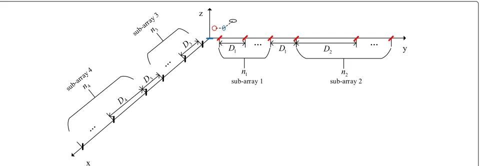
Figure2demonstrates our proposed array configuration
composed of an L-shaped sparse scalar array and a single triangular SS-EMVS. The triangular SS-EMVS is located at the origin and two scalar arrays are placed along the
x-axis andy-axis, respectively. The antennas on the two arms of the L-shaped array are oriented differently, i.e., along with ex and ez, respectively. Each arm of the L-shaped array consists of two sub-arrays. Taking the arm along with they-axis as an example, the first sub-array, which consists of the firstn1dipoles (including theex in the triangular SS-EMVS located at the origin), is placed with inter-sensor spacingD1 > x,y λ/2; the second sub-array, which consists of the lastn2dipoles, is placed
with an even larger inter-sensor spacing D2 = m1D1,
wherem1is an integer. Futhermore, we can see that the
first sub-array and the triangular SS-EMVS share a same
ex. Similarly, the arm of the L-shaped array along with the
x-axis consists of two sub-arrays with inter-sensor spac-ingsD3 > y,z λ/2 andD4 = m2D3, respectively,
wherem2is an integer; the first sub-array and the
Fig. 2The proposed array configuration. The triangular SS-EMVS in Fig.1is located at the origin.The scalar array whose unit isexis extended along
y-axis. The inter-sensor spacing in sub-array 1 isD1and the inter-sensor spacing in sub-array 2 isD2, respectively, whereD2=m1D1and
D1> x,yλ/2. Similarly, the scalar array whose unit isezis extended alongx-axis. The inter-sensor spacing in sub-array 3 isD3and the
inter-sensor spacing in sub-array 4 isD4, respectively, whereD4=m2D3andD3> y,zλ/2
different orientations, and they are the same as the dipoles of the triangular SS-EMVS along with the corresponding axis.
We take the scalar array placed along they-axis as the example again to illustrate the design idea of the proposed array. The triangular SS-EMVS can provide a coarse esti-mate ofvby applying the vector-cross-product algorithm. And the estimation result can be used as a reference for solving the ambiguity problem of thevestimate from the first sub-array in the scalar array. Therefore, the inter-sensor spacing of the first sub-array can be larger than λ/2. The aperture of the first sub-array is much larger than the inter-dipole/loop spacings of the triangular SS-EMVS and thus we can obtain a finer estimate of thevwith the first sub-array. Similarly, the disambiguated estimation result of the first sub-array can be adopted as the refer-ence of the second sub-array and finally a high-accuracy
vestimation result is obtained. Similarly, we can use the same method for the scalar array placed along thex-axis to obtain a high-accuracyuestimation result. Finally, the high-accuracy angular estimation results can be calcu-lated with the high-accuracyuandvestimations. Besides, the inter-sensor spacings of the two scalar arrays are much
larger than λ/2, and thus the apertures and the angle
estimation accuracy of the proposed array will be bet-ter than the L-shaped array withλ/2 inter-sensor spacing [31] and the L-shaped nested array [32] with λ/2 inter-sensor spacing in the first sub-array. These probabilities will be verified in Section4through extensive simulation experiments. In addition, owing to that the scalar arrays are extended alongx-axis andy-axis at the same time, 2D high-accuracy DOA estimations can be obtained simulta-neously. This can not be reached by the multi-scale EMVS array proposed in [21], where the multi-scale aperture extension is only in one axis. Furthermore, only a single
SS-EMVS (along with scalar sensors) instead of many SS-EMVSs are adopted in the proposed array, and thus the cost and redundancy of the array will be decreased dramatically.
2.3 Array manifold and signal model
The array manifold of the scalar array placed along they -axis is
where⊗denotes the Kronecker product,ais defined in
Eq. (1),a[ 1] is the first row ofa, and thusay∈CN1×1with
N1=n1+n2.
Similarly, the array manifold of the scalar array placed along thex-axis is
wherea[ 3] is the third row ofa, and ax ∈ CN2×1with
N2=n3+n4.
Following this, the array manifold of the proposed array is
In a multiple sources scenario withK incident signals, the received data of the proposed sparse array at timetis
x(t)= andn(t)signifies the additive white Gaussian noise.
ConsideringLtime snapshots, we can form the received data matrix
X=[x(t1),x(t2),. . .,x(tL)] . (8)
The following task is to estimate the DOA of these K
sources fromX∈CN×L, which will be described in detail below.
3 Procedure of multi-scale DOA estimation algorithm
As described in Section2.2, we can obtain multiple esti-mates of the direction cosines alongy-axis andx-axis by the received data of the triangular SS-EMVS and the two arms of the L-shaped array. However, some of the esti-mates are cyclically ambiguous and we will use the coarse estimates to disambiguate the ambiguous estimates step by step. The procedure of the entire algorithm is shown in Algorithm 1.
In the following, we give the detailed derivation and progress of the DOA estimation algorithm.
3.1 ESPRIT-based method to estimate thetwo setsof high-accuracy but cyclically ambiguousvandtwo sets
of high-accuracy but cyclically ambiguousu
The array covariance matrix can be calculated by the maximum likelihood estimation
ˆ R= 1
LXX
H, (9)
where the superscriptH is the Hermitian operator. Fol-lowing [4], letEs ∈ CN×K be the signal subspace matrix
composed of the K eigenvectors corresponding to the
K largest eigenvalues ofRˆ. AndEs has the same signal
Algorithm 1Proposed DOA estimation algorithm 1: Estimate thetwo sets of high-accuracy but cyclically
ambiguous y-axis direction cosine v estimations by the two sub-arrays placed along they-axis using the ESPRIT algorithm [33].
2: Estimate thetwo sets of high-accuracy but cyclically
ambiguous x-axis direction cosine u estimations by the two sub-arrays placed along thex-axis using the same method as mentioned in 1.
3: Estimate the unambiguous but low-accuracy y-axis
direction cosinevandx-axis direction cosineuas well as therelatively high-accuracy but ambiguous y-axis direction cosinevandx-axis direction cosineufrom the triangular SS-EMVS as in [11].
4: Disambiguate the ambiguousuandvestimates
pro-gressively and calculate the final (high-accuracy) arriving angles of the sources.
subspace with the manifold matrixBand thus
Es=BT, (10)
whereTdenotes an unknownK×Knon-singular matrix.
According to the composition of the proposed array, we divide the manifold matrix B into three parts, i.e., B1,
By, and Bx, where B1 ∈ C6×K is composed of the top
six rows ofB(corresponding to the triangular SS-EMVS), By∈CN1×Kis composed of the first row ofBand(N1−1)
rows from the seventh row (corresponding to the senors on they-axis), andBx ∈ CN2×K is composed of the third row ofBand(N2−1)rows from the(N1+5)th row
(cor-responding to the senors on thex-axis). In this way,B1,
By, andBxsignify the manifold matrices of the SS-EMVS and the two scalar arrays, respectively. Similarly, we can divide the signal subspace matrixEsinto three parts with the same method, i.e.,Es1,Esy, andEsx. Thus, according to the relationship between array manifold matrix and signal subspace [33] described in Eq. (10), we have
Es1 = B1T, (11)
Esy = ByT, (12)
Esx = BxT. (13)
After this, we deal with Esy and Esx separately to get two sets of the high-accuracy but cyclically ambiguous estimates of v and u. Let us take Esy as an example to demonstrate the derivation. According to the different inter-sensor spacings of the scalar array whose unit isex, we divide theEsy into two parts, i.e.,Esy,1 andEsy,2, where
Esy,1 ∈Cn1×K andEsy,2 ∈Cn2×K correspond to sub-array
1 and sub-array 2, respectively. Recalling Fig.2, both sub-array 1 and sub-sub-array 2 are uniform sub-arrays, so the ESPRIT algorithm can be used toEsy,1 andEsy,2 to obtain two sets
v, respectively. The process is consistent with that devel-oped in [21]. Since the inter-sensor spacingD1andD2are
both larger thanλ/2, two sets of high-accuracy but cycli-cally ambiguousy-axis direction cosine estimationsvˆfine,1k
andvˆfine,2k can be derived.
In addition, it can be seen from [21,34] that due to the same column permutation ofT, these two sets ofv estima-tions{ˆvfine, 1k }Kk=1and{ˆvfine, 2k }Kk=1are paired automatically. Besides, we can obtain two sets of high-accuracy but cyclically ambiguous u estimations, uˆfine,1k anduˆfine,2k by applying similar process to Esx. And the u estimations,
ˆ
ufine,1k anduˆfine,2k , are also paired automatically. 3.2 Vector-cross-product algorithm to estimate the
unambiguous but low-accuracy vanduand the
relatively high-accuracy but ambiguous vandu
According to [18,24], we need to get the estimate of the array manifold in order to apply the vector-cross-product algorithm to process the data of the triangle SS-EMVS.
And recalling Eq. (11), we can estimate the manifold
matrix of the SS-EMVS with
ˆ
andaˆkis the estimation of array manifold ofkth source at the triangular SS-EMVS.
The following step is to apply the vector-cross-product algorithm toaˆk. For convenience, we setθ ∈[ 0,π/2],φ ∈
According to the vector-cross product algorithm of the triangular SS-EMVS [11], we have,
p= (e˜)×(h˜)
where×denotes the vector-cross product andpis calcu-lated fromaˆ.
From the Poynting vector of kth source pk derived in Eq. (17), we can obtain theunambiguous but low-accuracy
estimations of{uk,vk,wk}by | |denotes the absolute value of the entity inside| |.
In the following, we estimate the relatively high-accuracy estimation ofuandvfrom the displacement of the dipoles/loops within the triangular SS-EMVS, i.e.,x,y andy,z. Fromp, we can get
wheredenotes the Hadamard (element-wise) product.
Based on Eq. (19), we have one set of relatively high-accuracy but ambiguousestimations ofuandvby
ˆ
It is worth mentioning that the unambiguous but low-accuracy estimations {ucoarsek }Kk=1 and the relatively high-accuracy but ambiguous estimations{ˆufine, 0k }Kk=1are paired automatically, and due to the sameTin Eq. (14), all
uestimations have been paired, the same forv. Moreover, forθ andφ in other angular ranges, the changes are the plus or minus signs in Eqs. (18) and (19) [11].
3.3 Disambiguate the estimations ofuandvand calculate the final estimates ofθandφ
As can be seen from the above Sections3.1and3.2, for both u and v, there are three sets of high-accuracy but ambiguous estimations and one set of unambiguous but low-accuracy estimation. The three sets of ambiguous estimations correspond to different levels of ambiguity, and a three-order disambiguation method is utilized here.
We take vas the example to demonstrate the
deriva-tion and the process foruis similar. Recalling Fig. 2, we know the ambiguity ofˆvfine,0k ,vˆfine,1k , andvˆfine,2k correspond tox,y,D1, andD2, respectively. And due to the fact that
D2>D1> x,y, the order of solving ambiguity should be ˆ
vfine,0k ,vˆfine,1k ,vˆfine,2k step by step.
3.3.1 Disambiguatevˆkfine,0with vkcoarse
Withvcoarsek as the reference value, the ambiguity ofvˆfine,0k
is solved, and the result can be obtained by
where−1− ˆvfine,0k x,y
with denoting the smallest integer not less than and
referring to the largest integer not more than [35].
3.3.2 Disambiguatevˆfine,1k with vfine, 0k
Withvfine, 0k as the reference value, the ambiguity ofˆvfine,1k
is solved, and the result can be obtained by
vfine, 1k = ˆvfine, 1k + ˆl2 λ
3.3.3 Disambiguatevˆfine,2k with vfine, 1k
Finally, we can disambiguate vˆfine,2k with vfine, 1k derived above to estimate the final high-accuracy and unambigu-ous estimation ofvfinalk :
vfinalk = ˆvfine, 2k + ˆl3 λ Similar to the above three steps, we can get the final high-accuracy and unambiguous estimation of ufinalk by replacing{x,y,D1,D2}with{y,z,D3,D4}, respectively.
After getting the unambiguous and high-accuracy
esti-mation of {u,v}, we can get the high-accuracy DOA
estimation ofkth source by (3) and the results are
⎧
3.4 Analysis of the three inter-sensor spacings
Larger inter-sensor spacing brings in larger aperture and further leads to higher direction estimation accuracy. At the same time, it makes the disambiguation more diffi-cult. There is a threshold in the process of disambiguation [36]. When the inter-sensor spacing value is larger than the threshold, the probability of successful disambiguation will break down. Therefore, we analyze the threshold of the inter-sensor spacing by analyzing the success proba-bility of the disambiguation process.
Let us takevas an example to demonstrate the deriva-tion again. According to the proposed array configuraderiva-tion shown in Fig.2, there are three scales, i.e.,{x,y,D1,D2}
forv. Thus, we utilize the three-order disambiguation pro-cess in Section 3.3 to obtainvfinal. Take the x,y as an example, recalling Eq. (23), only by satisfying the following equation
vrefk −vcoarsek < λ
2x,y
, (29)
can the disambiguation process be successful. The value ofvrefk −vcoarsek is the estimation error of thevcoarsek . We hereby assume that the angle estimation error follows a Gaussian distribution [37]. According to the distribution function of the normal process [38], the probability of the sample error falling into the scope of 3σ is about 99.85%, whereσ is the standard deviation of the samples. Thus, when the root mean square error (RMSE) ofvcoarsek
satisfies
we consider that the disambiguation process is successful. Therefore, we can calculate the threshold ofx,yby
threshold x,y =
λ 6σvcoarsek
. (31)
We can obtain the threshold ofD1 and D2 using the
similar method. Furthermore, considering the practical applications, we can only obtain the Cramér-Rao bounds (CRB) of each parameter rather than RMSE. Thus, we can substitute the RMSE ofvfine,0k andvfine,1k with their CRB to calculate the thresholds ofD1andD2. However, due to the
CRB is much less than the RMSE, the calculated values of thresholds ofD1andD2will be far larger than the actual
values. And this probility will be verified in Section4. Similar tov, we can obtain the corresponding thresholds of{y,z,D3,D4}foru.
Owing to the fact that RMSE is related to signal-to-noise ratio (SNR), the snapshot number and the source direction, we will analyze the influence of these factorsin Section4.
The derivation of the CRB for the new array is similar to that in [21], and we will use the corresponding equations therein to derive the CRB in the following simulations.
4 Simulation results and discussion
In this section, we conduct simulations to verify the effec-tiveness and performance of the proposed array geometry and algorithm. For simplicity, we set θ ∈[ 0,π/2], φ ∈ [ 0,π/2). The coordinate of the hy of the SS-EMVS is (xh,yh,zh) = (7.5λ, 7.5λ, 5λ). The RMSE of parameter estimation is defined as
RMSE=
Mis the number of Monte Carlo trials. We assume that
4.1 Parameter estimation results
In the first example, we consider that there areN1 = 12
ex’s placed along the y-axis direction andN2 = 12 ez’s placed along thex-axis direction. The first sixex’s
com-pose the sub-array 1 with inter-sensor spacing D1 =
35λ; the rest of the ex’s constitute the sub-array 2 with inter-sensor spacing D2 = 7D1 = 245λ. Besides, the
first six ez’s compose the sub-array 3 with inter-sensor spacingD3 = 35λ; the rest of theez’s constitute the
sub-array 4 with inter-sensor spacing D4 = 7D3 = 245λ.
For the triangular SS-EMVS, x,y = y,z = 5λ. There
areK = 2 pure-tone incident sources with unit power,
which have the numerical frequencyf = (0.537, 0.233),
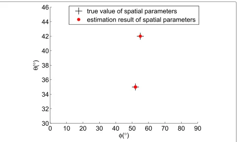
elevation θ = (42◦, 35◦), azimuth φ = (55◦, 52◦), the auxiliary polarization angleγ =(36◦, 60◦), and the polar-ization phase difference η = (80◦, 70◦) impinging on
the array. The number of snapshots is L = 200 and
SNR = 10 dB. The noise is a complex Gaussian white noise vector with zero mean and covariance matrixσ2I.
Figure 3 shows the estimation results of the proposed
algorithm with 200 Monte Carlo trials. We can see that the spatial parameters of all targets are correctly paired and estimated.
4.2 Parameter estimation performance
In order to further exploit the performance of the pro-posed array, we hereby conduct various simulations with different parameters of the array and sources.
4.2.1 Performance versus SNR
In the first example, we consider the performance of
parameter estimation versus SNR. Figure 4 a shows the
RMSE of all estimates of u, i.e., ufine,0, ufine,1, andufinal
of the proposed array versus SNR compared withucoarse
and the CRB. Figure 4 b shows the RMSE of all
esti-mates of v, i.e., vfine,0, vfine,1, and vfinal of the proposed array versus SNR compared withvcoarse and the CRB. It can be observed that both ufinal and vfinal improve sig-nificantly from their coarse estimates,ucoarseandvcoarse, respectively; both of them are getting closer to their CRB.
Moreover, the disambiguation described in Section 3.3
is similar to that of dual-size ESPRIT [4]. There exists a SNR threshold in the process of disambiguation [39]. The parameter estimation performance will be degraded significantly if the SNR is lower than the threshold. When SNR is larger than this threshold, the performance improves dramatically, and the performance is getting
bet-ter with the increase of SNR. From Fig. 4, we can see
that the SNR threshold of u and v are 7 dB and 6 dB,
respectively.
In addition, we compare the proposed array with the array configuration in [32] which has the same number of scalar sensors, and the array configuration in [21] which
has the same number of SS-EMVSs in y-axis. Figure 5
a and b shows the RMSE of u and v estimates versus
SNR for all three arrays, respectively. Comparing with the 2D nested scalar array in [32], the proposed array has a much larger aperture extension and lower mutual cou-pling; comparing with the linear multi-scale SS-EMVS array in [21], the proposed array has a much larger aper-ture extension inx-axis. We can observe from Fig.5a that the performance of the proposed array ofuestimation is higher than those of the two other arrays when SNR is larger than the threshold. That is because the array aper-ture of the proposed array inx-axis is much larger than the two other arrays. From Fig.5b, we can observe that the performance of the proposed array ofvestimation is a little worse than that of the array configuration in [21]. However, the SNR threshold of the proposed array is far smaller (7 dB).
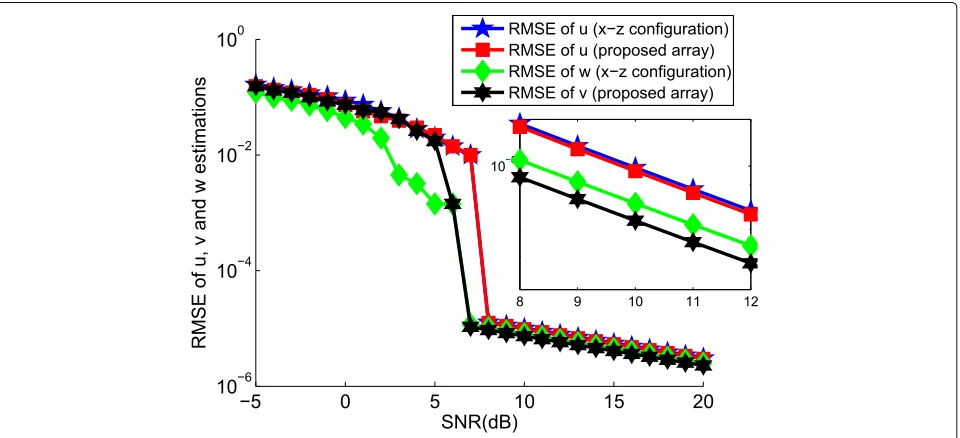
Moreover, we consider another configuration of the pro-posed array in which the array is extended alongy-axis and
z-axis, respectively. And the triangular SS-EMVS of this configuration is placed along y-axis and z-axis, respec-tively. The DOA estimation process of this array is similar to that of the proposed array, except that the
correspond-ing direction cosines change from u andv to v and w.
Using the same simulation conditions as in Section 4.1, we compare the parameter estimation performance of this array configuration with the proposed array. The results are given in Fig.6. We can observe that RMSEs ofu of these two configurations are similar, and the same behav-ior happens forvof the proposed array andwof another configuration. But we still can see that the accuracy of the proposed array are marginally better than the other configuration when SNR is large enough, i.e.,>8 dB.
As the arriving angle estimation is determined by u
andvjointly, in Fig. 7, we show the RMSEs of the
esti-mated θ and φ of all array configurations versus SNR
and the CRB of the proposed array. It can be seen that
the SNR threshold of θ and φ of the proposed array
are both 7 dB, the lowest one of the threshold of uand
v. Moreover, the performance of the proposed array is
the best in all array configurations. Therefore, our pro-posed array is a good trade-off of mutual coupling, esti-mation accuracy, and robustness (lower SNR threshold) to noise.
4.2.2 Performance versus snapshot number
In the next example, we consider the performance of
DOA estimation versus snapshot number L. Figure 8 a
and b show the RMSEs of θ and φ estimation of all
array configurations versus L at SNR=10 dB,
Fig. 3The estimation results of the DOA of two incident sources
4.2.3 Performance versus inter-sensor spacing
In the third example, we consider the performance of parameter estimation versus inter-sensor spacings. We take one target as an example, and set x,y = y,z
in the SS-EMVS with SNR=10 dB. The elevation of
the target is θ = 35◦, azimuth φ = 52◦, the
auxil-iary polarization angle γ = 36◦, and the polarization phase differenceη = 80◦. As mentioned in Section3.4, there is a threshold of inter-sensor spacing. Figure 9 shows the RMSE of ufine,0 and vfine,0 of the proposed
array versus x,y. Recalling Eq. (31), we can obtain the threshold of y,z at SNR=10 dB is ty,z = 7.15λ. From Fig. 9, the threshold of y,z is approximately 6λ. Thus, according to the obtained threshold and practical
applications, we sety,z = 5λ. The same method can
be performed forx,y, tx,y = 8.04λ, and the threshold of x,y is approximately 8λ from Fig. 9. Therefore, the method derived in Section3.4for calculating the thresh-olds of different inter-sensor spacings is effective. Similar toy,z, we setx,y=5λ.
Fig. 5RMSE ofuandvestimations of all three arrays versus SNR.aRMSE ofuestimations.bRMSE ofvestimations
In the second simulation, we set D1 = D3, and the
RMSE of ufine,1 andufine,1 of the proposed array versus
D1is shown in Fig.10. Similar toy,z, we can calculate the threshold ofD1andD3. But there is little different, as
mentioned in Section3.4, we utilize the CRB ofufine,0and
vfine,0instead of the RMSE to calculate the threshold ofD1
andD3. And the calculated value are Dt1 = 161.5λand
Dt3 = 197.5λ. From Fig.10, we can obtain these thresh-old values (Dt1 = 76λ,Dt3 = 72λ). We know that CRB is much smaller than RMSE. Therefore, we should setD1
andD3much smaller than the calculated threshold values.
Thereby, we setD1=D3=35λ.
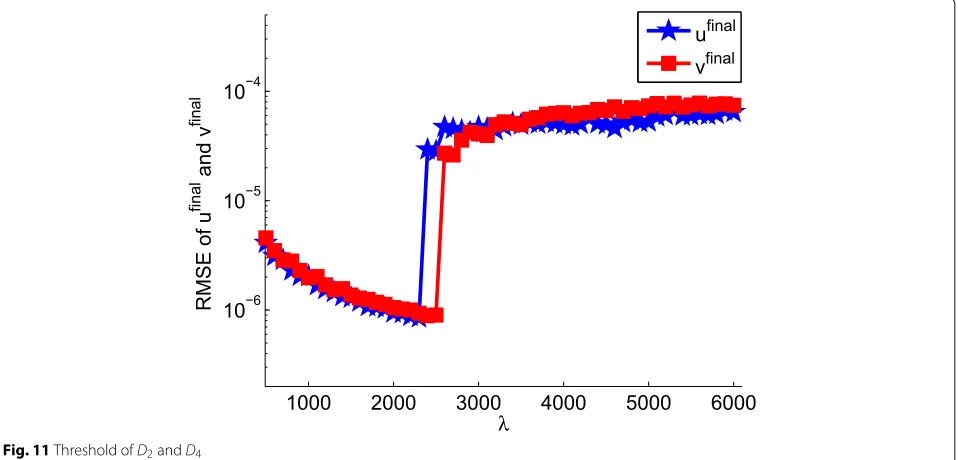
In the third simulation, we set D2 = D4and plot the
RMSE ofufinalandufinalof the proposed array versusD2
in Fig. 11. Similar toD1, we can calculate the threshold
of D2 and D4, Dt2 = 8047.6λ and Dt4 = 7857.9λ, by
CRB. From Fig. 11, we can obtain these threshold
val-ues !Dt2=2500λ,Dt4=2300λ". Again, we should setD2
much smaller than the calculated threshold values, and considering the practical applications, we setD2= D4 =
245λ.
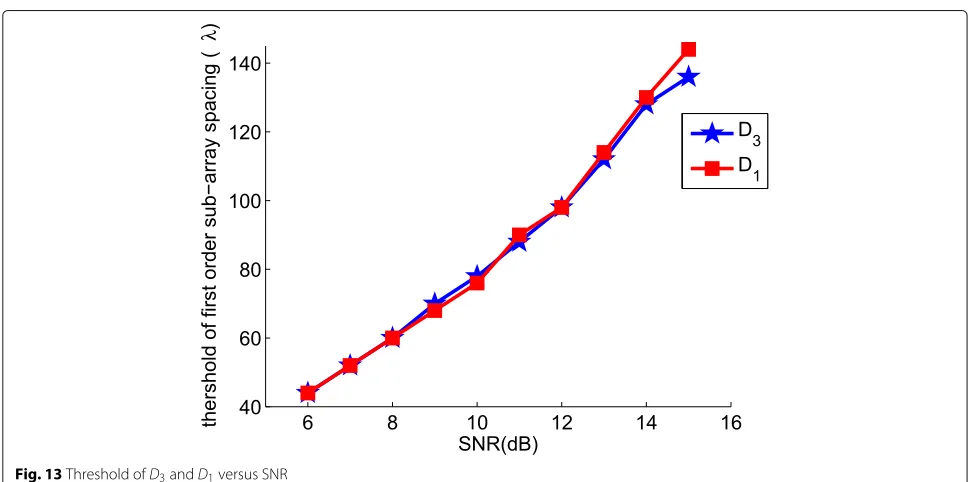
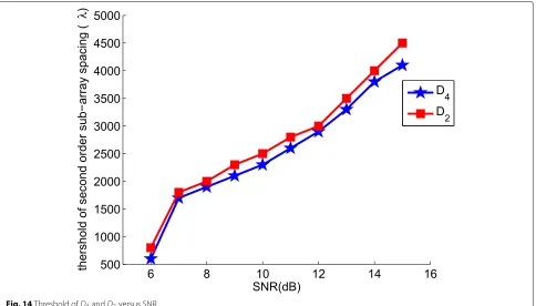
4.2.4 Threshold of inter-sensor spacing versus SNR
We investigate the threshold of inter-sensor spacing ver-sus SNR. Take one target as example, and we set the elevation of the target asθ = 35◦, azimuthφ = 52◦, the auxiliary polarization angleγ =36◦, and the polarization phase difference η = 80◦. Other simulation conditions
remain the same with Section 4.1. Figure 12shows the
thresholds of y,z and x,y versus SNR. It is seen that the thresholds of y,z and x,y both increases as SNR increases. And the thresholds of{D1,D3}and{D2,D4}are
Fig. 7RMSE ofθandφestimations versus SNR.aRMSE ofθestimations.bRMSE ofφestimations
Fig. 8RMSE ofθandφestimations versusL.aRMSE ofθestimations.bRMSE ofφestimations
Fig. 10Threshold ofD1andD3
shown in Figs. 13 and 14, respectively. The results are similar to Fig.12.
4.2.5 Threshold of SNR versus arriving angle
Lastly, we consider the threshold of SNR in the disam-biguation process versus the signal arriving angle. Take one target as the example, we set the auxiliary
polariza-tion angle of the target γ = 36◦ and the polarization
phase differenceη=80◦. We set another angle equals 45◦ when we analyze one angle. Other simulation conditions remain the same as in Section4.1. Figure 15 shows the
threshold of SNR ofuandvversusθ andφ. We can see that the threshold of SNR is approximately symmetrical with 90◦forθ and symmetrical with 0◦forφ. As we set θ ∈[ 0,π/2] andφ ∈[ 0,π/2), the threshold of SNR is in a lower range when the target is located inθ ∈[ 20◦, 70◦] andφ ∈[ 20◦, 70◦].
5 Conclusions
In this paper, a new array configuration composed of multiple sparse scalar arrays and a single trian-gle electromagnetic-vector-sensor is proposed, which
Fig. 12Threshold ofy,zandx,yversus SNR
enjoys the superiorities of both the spatially spread electromagnetic-vector-sensor and the sparse array. The new array can provide four direction cosine estimates with gradually improved accuracies, which are along the x-axis and y-axis, respectively. Based on this, we developed the algorithm for direction-of-arrival estima-tion, which utilizes the approach of three-order dis-ambiguation. We have analyzed the thresholds of the inter-sensor spacings in the four uniform scalar sub-arrays and conducted extensive simulations to validate
them. We compare the performance of the direction cosine estimations of our array with the 2D nested scalar array and the linear multi-scale SS-EMVS array. These results demonstrated that our proposed array geome-try enjoys the optimal trade-off on estimation accuracy, mutual coupling, and robustness to noise. Moreover, since only a single SS-EMVS is used with other scalar sensors, the proposed array has achieved a good per-formance with small redundancy, less elements, and low cost.
Fig. 14Threshold ofD4andD2versus SNR
Abbreviations
2D: Two-dimensional; DOA: Direction-of-arrival; DOF: Degree-of-freedom; CRB: Cramér-Rao bounds; EMVS: Electromagnetic-vector-sensor; ESPRIT: Estimation of signal parameters via rotation invariant technique; RMSE: Root mean square error; SS-EMVS: Spatially spread electromagnetic-vector-sensor; ULAs: Uniform linear arrays
Acknowledgements
This work is partly supported by the National Natural Science Foundation of China under Grant 61571344, in part by the Foundation of Shanghai Academy of Spaceflight Technology under Grant SAST2016093 and in part by the Fund for Foreign Scholars in University Research and Teaching Programs the 111 Project under Grant B18039.
Authors’ contributions
JD, MLY, BXC, and XY conceived and designed the study. JD and MLY performed the experiments. JD and MLY wrote the paper. MLY, BXC, and XY reviewed and edited the manuscript. All authors read and approved the manuscript.
Competing interests
The authors declare that they have no competing interests.
Author details
1National Laboratory of Radar Signal Processing, Xidian University, Xi’an, China. 2Nokia Bell Labs, Murray Hill, USA.
Received: 26 February 2019 Accepted: 26 August 2019
References
1. H. L. Van Trees,Optimum Array Processing: Part IV of Detection, Estimation, and Modulation Theory. (John Wiley & Sons, New York, 2004)
2. X. Yuan, Direction-finding wideband linear fm sources with triangular arrays. IEEE Trans. Aerosp. Electron. Syst.48(3), 2416–2425 (2012) 3. K. T. Wong, M. D. Zoltowski, inProceedings of the 39th Midwest Symposium
on Circuits and Systems. Sparse Array Aperture Extension with Dual-Size Spatial Invariances for ESPRIT-based Direction Finding (IEEE, IA, 1996), pp. 691–6942
4. V. I. Vasylyshyn, inEuropean Radar Conference, 2005. Unitary ESPRIT-based DOA estimation using sparse linear dual size spatial invariance array (IEEE, Paris, 2005), pp. 157–160
5. A. L. Swindlehurst, B. Ottersten, R. Roy, T. Kailath, Multiple invariance ESPRIT. IEEE Trans. Signal Process.40(4), 867–881 (1992)
6. A. Moffet, Minimum-redundancy Linear Arrays. Antennas Propag. IEEE Trans.16(2), 172–175 (1968)
7. P. Pal, P. P. Vaidyanathan, Nested arrays: A novel approach to array processing with enhanced degrees of freedom. Signal Process. IEEE Trans.
58(8), 4167–4181 (2010)
8. P. P. Vaidyanathan, P. Pal, Sparse sensing With co-prime samplers and arrays. Signal Process. IEEE Trans.59(2), 573–586 (2011)
9. A. Nehorai, P. Tichavsky, Cross-product algorithms for source tracking using an EM vector sensor. IEEE Trans. Signal Process.47(10), 2863–2867 (1999) 10. X. Yuan, Estimating the DOA and the polarization of a polynomial-phase
signal using a single polarized vector-sensor. IEEE Trans. Signal Process.
60(3), 1270–1282 (2012)
11. X. Yuan,Diversely polarized antenna-array signal processing. PhD thesis. (The Hong Kong Polytechnic University, 2012)
12. X. Yuan, in2012 IEEE International Conference on Acoustics, Speech and Signal Processing (ICASSP). Polynomial-phase signal source tracking using an electromagnetic vector-sensor, (Kyoto, 2012), pp. 2577–2580 13. X. Yuan, K. T. Wong, Z. Xu, K. Agrawal, Various compositions to form a triad
of collocated dipoles/loops, for direction finding and polarization estimation. IEEE Sensors J.12(6), 1763–1771 (2012)
14. X. Yuan, Quad compositions of collocated dipoles and loops: For direction finding and polarization estimation. IEEE Antennas Wirel. Propag. Lett.11, 1044–1047 (2012)
15. X. Yuan, K. T. Wong, K. Agrawal, Polarization estimation with a dipole-dipole pair, a dipole-loop pair, or a loop-loop pair of various orientations. IEEE Trans. Antennas Propag.60(5), 2442–2452 (2012) 16. Z. Xu, X. Yuan, Cramer-Rao bounds of angle-of-arrival and polarisation
estimation for various triads. IET Microw. Antennas Propag.6(15), 1651–1664 (2012)
17. K. T. Wong, M. D. Zoltowski, Uni-vector-sensor ESPRIT for multisource azimuth, elevation, and polarization estimation. IEEE Trans. Antennas Propag.45(10), 1467–1474 (1997)
18. K. T. Wong, X. Yuan, ‘Vector cross-product direction-finding’ with an electromagnetic vector-sensor of six orthogonally oriented but spatially noncollocating dipoles/loops. IEEE Trans. Signal Process.59(1), 160–171 (2011)
19. X. Yuan, in2011 IEEE Statistical Signal Processing Workshop (SSP). Cramer-Rao bound of the direction-of-arrival estimation using a spatially spread electromagnetic vector-sensor, (Nice, 2011), pp. 1–4
20. X. Yuan, Spatially spread dipole/loop quads/quints: For direction finding and polarization estimation. IEEE Antennas Wirel. Propag. Lett.12, 1081–1084 (2013)
21. M. Yang, J. Ding, B. Chen, X. Yuan, A multiscale sparse array of spatially spread electromagnetic-vector-sensors for direction finding and polarization estimation. IEEE Access.6, 9807–9818 (2018)
22. X. Yuan, Coherent sources direction finding and polarization estimation with various compositions of spatially spread polarized antenna arrays. Signal Process.102, 265–281 (2014)
23. F. Luo, X. Yuan, Enhanced ‘vector-cross-product’ direction-finding using a constrained sparse triangular-array. EURASIP J. Adv. Signal Process.
2012(1) (2012).https://doi.org/10.1186/1687-6180-2012-115 24. Y. Li, J. Q. Zhang, An enumerative nonlinear programming approach to
direction finding with a general spatially spread electromagnetic vector sensor array. Signal Process.93(4), 856–865 (2013)
25. X. Yuan, Spatially spread dipole/loop quads/quints: For direction finding and polarization estimation. IEEE Antennas Wirel. Propag. Lett.12, 1081–1084 (2013)
26. M. Ji, X. Gong, Q. Lin, in2015 12th International Conference on Fuzzy Systems and Knowledge Discovery (FSKD). A multi-set approach for direction finding based on spatially displaced electromagnetic vector-sensors (IEEE, Zhangjiajie, 2015), pp. 1824–1828
27. K. Han, A. Nehorai, Nested vector-sensor array processing via tensor modeling. IEEE Trans. Signal Process.62(10), 2542–2553 (2014) 28. J. He, Z. Zhang, T. Shu, W. Yu, Direction finding of multiple partially
polarized signals with a nested cross-diople array. IEEE Antennas Wirel. Propag. Lett.16, 1679–1682 (2017)
29. S. Rao, S. P. Chepuri, G. Leus, in2015 IEEE 6th International Workshop on Computational Advances in Multi-Sensor Adaptive Processing (CAMSAP). DOA estimation using sparse vector sensor arrays (IEEE, Cancun, 2015), pp. 333–336
30. X. Yuan, Coherent source direction-finding using a sparsely-distributed acoustic vector-sensor array. IEEE Trans. Aerosp. Electron. Syst.48, 2710–2715 (2012)
31. J. Liang, D. Liu, Joint elevation and azimuth direction finding using L-shaped array. IEEE Trans. Antennas Propag.58(6), 2136–2141 (2010) 32. C. Niu, Y. Zhang, J. Guo, Interlaced double-precision 2-D angle estimation
algorithm using L-shaped nested arrays. IEEE Signal Process. Lett.23(4), 522–526 (2016)
33. R. Roy, T. Kailath, ESPRIT-Estimation of signal parameters via rotational invariance techniques. Acoust. Speech Signal Process. IEEE Trans.37(7), 984–995 (1989)
34. J. Li, M. Shen, D. Jiang, in2016 IEEE 5th Asia-Pacific Conference on Antennas and Propagation (APCAP). DOA estimation based on combined ESPRIT for co-prime array (IEEE, Kaohsiung, 2016), pp. 117–118
35. V. I. Vasylyshyn, inFirst European Radar Conference, 2004. EURAD. Closed-form DOA estimation with multiscale unitary ESPRIT algorithm (IEEE, Amsterdam, 2004), pp. 317–320
36. F. Athley, Threshold region performance of maximum likelihood direction of arrival estimators. IEEE Trans. Signal Process.53(4), 1359–1373 (2005) 37. B. Ottersten, M. Viberg, T. Kailath, Performance analysis of the total least
squares ESPRIT algorithm. IEEE Trans. Signal Process.39(5), 1122–1135 (1991) 38. D. C. Montgomery, G. C. Runger,Applied Statistics and Probability for
Engineers. (John Wiley & Sons, New York, 2010)
39. C. D. Richmond, Mean-Squared Error and Threshold SNR Prediction of Maximum-Likelihood Signal Parameter Estimation With Estimated Colored Noise Covariances. IEEE Trans. Inf. Theory.52(5), 2146–2164 (2006)
Publisher’s Note
![Fig. 1 Configuration of the triangular SS-EMVS [11]. The source is located at elevation angle θ and azimuth angle φ](https://thumb-us.123doks.com/thumbv2/123dok_us/879356.1105672/3.595.59.293.511.727/configuration-triangular-emvs-source-located-elevation-angle-azimuth.webp)