Resampling procedures to identify important SNPs using a consensus approach

P R O C E E D I N G S

Open Access

Resampling procedures to identify important

SNPs using a consensus approach

Christopher Pardy

, Allan Motyer

, Susan Wilson

From

Genetic Analysis Workshop 17

Boston, MA, USA. 13-16 October 2010

Abstract

Our goal is to identify common single-nucleotide polymorphisms (SNPs) (minor allele frequency > 1%) that add predictive accuracy above that gained by knowledge of easily measured clinical variables. We take an algorithmic approach to predict each phenotypic variable using a combination of phenotypic and genotypic predictors. We perform our procedure on the first simulated replicate and then validate against the others. Our procedure performs well when predicting Q1 but is less successful for the other outcomes. We use resampling procedures where possible to guard against false positives and to improve generalizability. The approach is based on finding a consensus regarding important SNPs by applying random forests and the least absolute shrinkage and selection operator (LASSO) on multiple subsamples. Random forests are used first to discard unimportant predictors, narrowing our focus to roughly 100 important SNPs. A cross-validation LASSO is then used to further select variables. We combine these procedures to guarantee that cross-validation can be used to choose a shrinkage parameter for the LASSO. If the clinical variables were unavailable, this prefiltering step would be essential. We perform the SNP-based analyses simultaneously rather than one at a time to estimate SNP effects in the presence of other causal variants. We analyzed the first simulated replicate of Genetic Analysis Workshop 17 without knowledge of the true model. Post-conference knowledge of the simulation parameters allowed us to investigate the limitations of our approach. We found that many of the false positives we identified were substantially correlated with genuine causal SNPs.

Background

Our goal is to identify single-nucleotide polymorphisms (SNPs) that add predictive information for the phenotypic outcomes above that given by just the other phenotypes. This aim is motivated by the use of genetic testing in a clinical setting, where SNP genotypes can be used to iden-tify a patient’s risk level better than easily measured clini-cal variables alone [1].

Our approach combines several well-known statistical procedures: stability selection, random forests, the least absolute shrinkage and selection operator (LASSO), and logistic regression. Random forests are an algorithmic machine learning technique based on a majority vote among a number of randomly varying trees [2,3]. The

algorithm generally gives good predictive accuracy at the expense of interpretability. It has the useful property of providing an importance score for each variable deter-mined by how worse prediction becomes when the given variable is removed from the analysis. This score allows us to add an additional filtering step at the outset to remove SNPs that do not provide useful predictive information. The importance score is insensitive to correlation or coli-nearity between variables (for example, see section 11.1 of Breiman [4]), allowing us to ignore linkage effects until a smaller set of variables is under consideration. Because of its good computational speed, we use the Random Jungle software, which was developed for a previous Genetic Analysis Workshop [3,5,6].

The LASSO procedure is a well-regarded approach to variable shrinkage and selection [3,7,8]. Although the required tuning parameter can be chosen by cross vali-dation [9], in our experience too many uninformative * Correspondence: [email protected]

1

Prince of Wales Clinical School, Faculty of Medicine, University of New South Wales, Sydney, New South Wales 2052, Australia

Full list of author information is available at the end of the article

variables can result in the lack of a global minimum deviance, thus making this parameter difficult to use. Our initial use of random forests minimizes this problem.

Multicolinearity causes regression models to fail, so we follow the example set by the authors of the PLINK software [5] and filter data based on variance inflation factors (VIFs). Population substructure can also be an issue [10], and we briefly investigated this using princi-pal components analysis.

To help protect against false positives and improve the generalizability of results, we use a consensus approach involving multiple subsamples. Subsamples (without replacement) from a single trial may give estimates with improved stability [11]. It has been suggested that sam-ples of sizen/2 perform well [11].

The true simulation model is described by Blangero et al. [12]. An overview of the use of machine learning methods in genetic epidemiology is given by Dasgupta et al. [3].

Methods

Combination of approaches

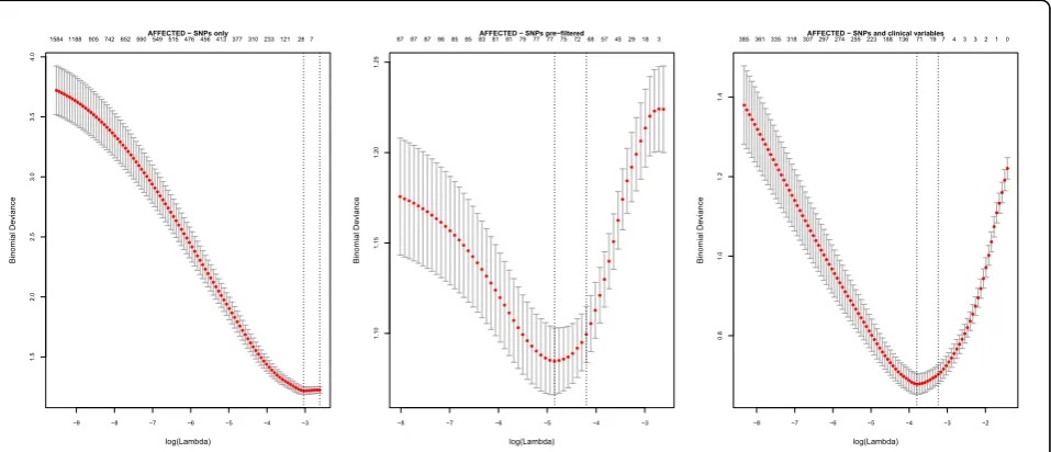
When preliminary analyses were confined to the SNPs only as predictors, we found that the LASSO procedure was unable to find a global minimum cross-validation error to select the shrinkage parameter (left-hand panel of Figure 1). Our use of random forests to prefilter the SNPs was driven by the need to find a minimum error (center panel of Figure 1). Alternatively, adjustment for clinical variables also achieved this (right-hand panel of

Figure 1). We applied the random forest importance scores first because this procedure does not exclude mul-tiple correlated variables. Because the LASSO assumes independent predictors, we removed highly correlated variables by means of VIF filtering.

Procedure

We removed SNPs that had a minor allele frequency (MAF) less than 0.01 or that failed a Hardy-Weinberg equilibrium test, leaving 4,755 SNPs for analysis. Random samples of size 348 were taken without replacement from the 679 subjects in the first replicate of the Genetic Analy-sis Workshop 17 (GAW17) data set. This procedure was repeated 10 times, with subsequent analyses performed on each subsample. We used a principal components analysis to investigate possible population structure within the SNPs and identified three clear groups that corresponded almost exactly with the three major ethnic groups of the subjects (African, Asian, and European). Many analyses were performed both with and without adjusting for ethni-city to determine whether this was an important confoun-der. In general, we found that ethnicity effects disappeared once the SNPs were taken into account (interestingly, a random forest fitted to the SNP data could perfectly pre-dict these ethnicity groups).

We applied the following procedure to each of the sub-samples (see Figure 2): (1) We used the Random Jungle program to perform a random forest analysis with 1,000 trees and a sample of 1,000 variables at each node. We assessed variable importance using the gene identification by NMD (nonsense mediated decay) inhibition (GINI)

−9 −8 −7 −6 −5 −4 −3

AFFECTED − SNPs and clinical variables

log(Lambda)

index, which largely matched other calculated impor-tance indexes. (2) We counted the number of times each variable appeared in the 100 most important variables. (3) We chose a cutoff to reduce the set of variables,

guided by the upper quartile of inclusion counts. A cutoff resulting in a set of roughly 100 SNPs was found to work well for subsequent stages. (4) Variables were iteratively dropped until none had a VIF greater than 10 when

!"#

"

$

%!&$ ' ()

$ *+,

& ())

regressed on the others. Because of the lack of substantial pairwise correlation between SNPs, few variables were dropped at this stage. (5) Within each replicate, we used cross validation to choose an appropriate penalty factor for the LASSO. This was done with the cv.glmnet() func-tion in the glmnet R package [9]. The“minimum MSE + 1 standard error”rule was most frequently found to lead to models that were sufficiently sparse to not obviously overfit the data. The random forest filtering step was necessary to ensure a global minimum model-fitting error in the cross-validation step. (6) We counted the number of times each variable was included in each LASSO model (i.e., the number of times each variable had a nonzero estimated coefficient). (7) We chose another cutoff. Once again, the upper quartile was found to be a good choice. (8) Finally, we fitted an unpenalized linear or logistic regression model using all 697 subjects. We used Bayesian information criterion (BIC) backwards selection to remove variables that did not contribute to the model fit. The LASSO step ensured that the maximal model at this stage (before backwards selection) had non-zero deviance and minimized the chance that fitted prob-abilities were 0 or 1.

We assessed the predictive accuracy over the 200 replicates of the GAW17 data set using the mean-square error (for continuous variables) or the proportion of incorrect predictions (for affected status). Models were fitted both with and without the SNPs to assess whether their inclusion improved accuracy.

Results Predicting Q1

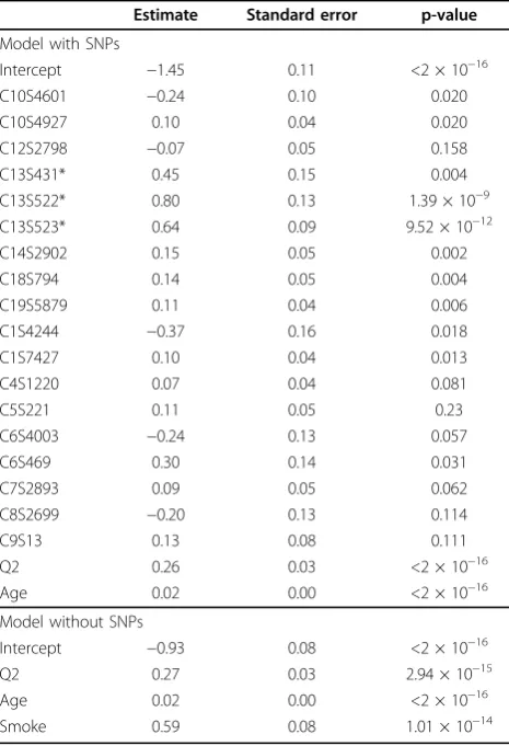
By far the most successful application of our procedure was the prediction of Q1. We observed how frequently SNPs were among the 100 most important variables iden-tified by the random forest. Only 2 SNPs appeared in all 10 subsamples (C13S522 and C13S523). Keeping variables that appeared at least three times (the upper quartile of this distribution) left 90 remaining SNPs. Checking the VIFs caused one SNP to be dropped to avoid colinearity. Similarly, we observed how frequently each variable remained in the model after a subsequent LASSO selec-tion. The upper quartile of this distribution was four, which was used as a cutoff for inclusion in the final model. We fitted a linear regression using the remaining vari-ables. After BIC backwards selection, we arrived at the “Model with SNPs”in Table 1. These fitted coefficients were used to predict Q1 in each of the other replicates. This gave a set of 199 mean-square prediction errors over the remaining replicates (including the first repli-cate). We used the median of these as a robust indication of model performance: 0.6899. We refitted the model without the SNPs and similarly validated it, finding a median mean-square error of 0.9868 (Table 1,“Model

without SNPs”). This demonstrates that a substantial reduction in prediction error can result from including the identified SNPs, suggesting that we found a set of SNPs with good predictive value.

Post-conference comparisons

Because Q1 was the most amenable to prediction, we decided to use this trait to compare various approaches in light of the true simulated model. To assess the effect of false positives, we fitted a model using only the three SNPs on chromosome 13 known to be casual (with Q1, Age, and Smoke) and found a median mean-square error of 0.6460 over the replicates. In addition, we compared these three SNPs to those SNPs chosen by a simple one-SNP-at-a-time genome-wide association approach with Bonferroni correction. The chosen SNPs were C12S707, C12S711, C12S2028, C12S2798, C13S522, and C13S523 (the chromosome 13 SNPs are genuinely causal). This model had a median mean-square error of 0.6651, with a slight performance improvement over our consensus approach.

Table 1 Final consensus models for Q1 with and without SNPs

Estimate Standard error p-value

Model with SNPs

Intercept −1.45 0.11 <2 × 10−16

C10S4601 −0.24 0.10 0.020

C10S4927 0.10 0.04 0.020

C12S2798 ₋0.07 0.05 0.158

C13S431* 0.45 0.15 0.004

C13S522* 0.80 0.13 1.39 × 10−9

C13S523* 0.64 0.09 9.52 × 10−12

C14S2902 0.15 0.05 0.002

C18S794 0.14 0.05 0.004

C19S5879 0.11 0.04 0.006

C1S4244 −0.37 0.16 0.018

C1S7427 0.10 0.04 0.013

C4S1220 0.07 0.04 0.081

C5S221 0.11 0.05 0.23

C6S4003 −0.24 0.13 0.057

C6S469 0.30 0.14 0.031

C7S2893 0.09 0.05 0.062

C8S2699 −0.20 0.13 0.114

C9S13 0.13 0.08 0.111

Q2 0.26 0.03 <2 × 10−16

Age 0.02 0.00 <2 × 10−16

Model without SNPs

Intercept −0.93 0.08 <2 × 10−16

Q2 0.27 0.03 2.94 × 10−15

Age 0.02 0.00 <2 × 10−16

Smoke 0.59 0.08 1.01 × 10−14

Predicting Q2, Q4, and affected status

The analysis to predict the traits Q2, Q4, and affected status was less successful. Although our procedure was motivated by the attempted analysis of affected status, we were unable to find a model that substantially reduced prediction error. This was also the case for Q2 and Q4, although we did identify a true causal SNP for Q2 (C6S5449).

Discussion and conclusions

We found that SNPs added predictive information only when Q1 was used as the outcome. Removing SNPs with a low MAF left Q1 as the only outcome that had common enough variants with large enough effect sizes for our approach to be successful. Many of the effect sizes seen in the true simulated model were so small as to be often overshadowed by spurious associations (evi-denced by the noncausal SNPs with smaller p-values than genuine causal ones).

It is interesting to note that only 15 of the true causal SNPs were included in our analysis after MAF filtering, and only 4 of these were in the top 100 important SNPs from the random forest plot (predicting Q1). These four SNPs correspond to the four correctly identified SNPs. Although one SNP is in the model to predict Q2, this variable is itself associated with Q1 (with an observed correlation of 0.24 in the first replicate). All true identi-fied SNPs had a MAF less than 3%. The choice of using 1,000 variables at each node in the random forest was confirmed by a separate cross-validation study. With hindsight it appears that this was required to ensure that the SNPs with strong effect (on chromosome 13) were selected often enough to reduce prediction error.

We had hoped that the consistent use of resampling-based procedures would stop overfitting of the models on the first replicate. This worked to the extent that pre-diction accuracy did not become substantially worse by including SNPs for any of the outcomes. The use of sub-sampling was preferred over simple cross validation because it gave a larger sample size (n/2) for each train-ing set with the ability to increase stability by taktrain-ing more subsamples. However, it would be preferable to have objective criteria for deciding whether a variable should be included at each stage rather than accepting the choices we were forced to make based on computa-tional tractability.

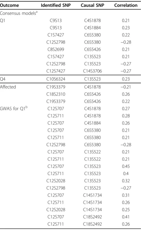
To explain some of the false positives, we calculated correlations between genuine causal SNPs for the con-sensus model and the naive genome-wide association study (Table 2). Many SNPs identified in our analyses had substantial observed correlations (using our linear SNP coding) greater than 0.2, nearly always across chro-mosomes. The correlation between SNPs on chromo-some 12 and those on chromochromo-some 4 (causal for Q1)

potentially explain the cluster of false positives picked up by the genome-wide association study. Many SNPs picked up by the consensus approach were correlated with causal SNPs. The multiple-SNP analysis of our consensus approach minimized this to a reasonable degree, identifying only a single SNP on chromosome 12. Because of our success in predicting Q1, we cannot conclude that the use of random forests as a prefiltering step is completely without merit. If the clinical variables were unavailable, this approach would allow the LASSO model to be fitted.

Acknowledgments

This research was funded by Australian National Health and Medical Research Council grant 525453. The Genetic Analysis Workshop is supported by National Institutes of Health grant R01 GM031575.

This article has been published as part ofBMC ProceedingsVolume 5 Supplement 9, 2011: Genetic Analysis Workshop 17. The full contents of the

Table 2 Strongest correlations between false positives and genuine causal SNPs

Outcome Identified SNP Causal SNP Correlation

Consensus modelsa

Q1 C9S13 C4S1878 0.21

C9S13 C4S1884 0.23

C1S7427 C6S5380 0.22

C12S2798 C6S5380 ₋0.28

C8S2699 C6S5426 0.21

C1S7427 C13S523 0.21

C12S2798 C13S523 −0.27

C12S7427 C14S3706 −0.27

Q4 C10S6324 C13S523 0.23

Affected C19S3379 C4S1878 −0.21

C18S2310 C6S5426 0.26

C19S3379 C6S5426 0.22

GWAS for Q1b C12S707 C4S1878 0.27

C12S711 C4S1878 0.28

C12S707 C4S1884 0.26

C12S707 C6S5380 0.21

C12S711 C6S5380 0.21

C12S2798 C6S5380 −0.28

C12S707 C13S522 0.21

C12S711 C13S522 0.21

C12S707 C13S523 0.45

C12S711 C13S523 0.4

C12S2028 C13S523 0.32

C12S2798 C13S523 −0.27

C12S707 C14S1734 0.31

C12S711 C14S1734 0.26

C12S2028 C14S1734 0.25

C12S707 C18S2492 0.41

C12S711 C18S2492 0.26

a

SNPs identified by our procedure.

b

supplement are available online at http://www.biomedcentral.com/1753-6561/5?issue=S9.

Author details

1

Prince of Wales Clinical School, Faculty of Medicine, University of New South Wales, Sydney, New South Wales 2052, Australia.2_{School of}

Mathematics and Statistics, Faculty of Science, University of New South Wales, Sydney, New South Wales 2052, Australia.

Authors’contributions

CP carried out the analysis and writing of the paper under the guidance of SW. AM provided the filtered dataset and helpful suggestions.

Competing interests

The authors declare that there are no competing interests.

Published: 29 November 2011

References

1. Humphries SE, Ridker PM, Talmud PJ:Genetic testing for cardiovascular disease susceptibility: a useful clinical management tool or possible misinformation?Arterioscler Thromb Vasc Biol2004,24:628. 2. Breiman L:Random forests.Machine Learning2001,45:5-32.

3. Dasgupta A, Sun YV, Konig IR, Bailey-Wilson JE, Malley JD:Brief review of machine learning methods in genetic epidemiology: the GAW17 experience.Genet Epidemiol2011,X(suppl X):X-X.

4. Breiman L:Statistical modeling: the two cultures.Stat Sci2001, 16:199-231, (with comments and a rejoinder by the author). 5. Purcell S, Neale B, Todd-Brown K, Thomas L, Ferreira MAR, Bender D,

Maller J, Sklar P, de Bakker PIW, Daly MJ,et al:PLINK: a tool set for whole-genome association and population-based linkage analyses.Am J Hum Genet2007,81:559-575.

6. Schwarz DF, Konig IR, Ziegler A:On safari to Random Jungle: a fast implementation of random forests for high dimensional data. Bioinformatics2010,26:1752-1758.

7. Hastie T, Tibshirani R, Friedman JH:The Elements of Statistical Learning: Data Mining, Inference, and Prediction.New York, Springer; 2009. 8. Tibshirani R:Regression shrinkage and selection via the Lasso.J R Stat

Soc Ser B Methodol1996,58:267-288.

9. Friedman J, Hastie T, Tibshirani R:Regularization paths for generalized linear models via coordinate descent.J Stat Softw2010,33:1-2210. 10. Price AL, Patterson NJ, Plenge RM, Weinblatt ME, Shadick NA, Reich D:

Principal components analysis corrects for stratification in genome-wide association studies.Nat Genet2006,38:904-909.

11. Meinshausen N, Buhlmann P:Stability selection.J Roy Stat Soc Ser B Stat Meth2010,72:417-473.

12. Almasy LA, Dyer TD, Peralta JM, Kent JW Jr, Charlesworth JC, Curran JE, Blangero J:Genetic Analysis Workshop 17 mini-exome simulation.BMC Proc2011,5(suppl 9):S2.

doi:10.1186/1753-6561-5-S9-S59

Cite this article as:Pardyet al.:Resampling procedures to identify important SNPs using a consensus approach.BMC Proceedings20115 (Suppl 9):S59.

Submit your next manuscript to BioMed Central and take full advantage of:

• Convenient online submission

• Thorough peer review

• No space constraints or color figure charges

• Immediate publication on acceptance

• Inclusion in PubMed, CAS, Scopus and Google Scholar

• Research which is freely available for redistribution