Reconstruction of 3D PIV data in complicated experimental arrangements

a

Ing. David Pavlík: [email protected]

Reconstruction of 3D PIV data in complicated experimental

arrangements

David Pavlík1, Václav Uruba2, Václav Kopecký1

1

Institute of New Technologies, Technical Univesity of Liberec, Studentská 2, Liberec, Czech Republic

2_{Institute of Termomechanics of the Academy of Sciences of the Czech Republic, Dolejšova 5, Praha 8, Czech Republic}

Abstract. In this paper a three-dimensional reconstruction of flow field behind flat plate representing a wing is presented. The reconstruction is always performed for pair of 2D vector maps obtained by 3D PIV with two cameras which record measurement area from different locations. Three-dimensional reconstruction can be obtained in various ways. This paper summarizes two: the reconstruction based on the known correspondences and the reconstruction based on the knowledge of intrinsic and extrinsic parameters of cameras. The methods can be used in the cases when it is impossible to use a calibration pattern or when reconstruction by commercial software fails.

1 Introduction

The 3D PIV is a contactless measurement method which is advisable to use for the comprehensive description actions behind flat plate with rounded edges. The method is based on the records of displacements of seeding particles carried by the fluid stream. Satiating particles are very small and their ideal size or other properties are determined by many experiments. During a measurement pulsed lasers are used in order to illuminate particles in predetermined measuring area. For recording of the particle images two cameras are mostly used. The optimal angle between axies of the cameras lens is 90º [1]. Two sets of images are used for computation of two-dimensional vector maps of flow field corresponding to each camera. The first set is captured at the time t while second set of images is recorded several microseconds later (t+t). The calculation is based on correlation methods. Subsequently, there are reconstructed 3D vector maps from the two-dimensional vector maps, which characterize fluid flow in the measurement area. The reconstruction can be done in several ways.

A calibration procedure of stereo-view has to precede each measurement. The calibration can be done based on the knowledge of geometry layout and parameters of cameras or by recording of a calibration pattern. The calibration pattern may be a plate with black/white dots on white/black background and with defined dimensions, see Fig. 4. This type of pattern is firstly recorded in the place of the laser cut and furthermore in several positions in front of the cut and behind the cut, see in paragraph 2.1. Another possibility is the calibration pattern in the form of a chessboard, which is positioned and recorded in place of the laser cut, as in the previous case, and is turned into random positions around the laser cut. The calibration pattern called multilevel target is another

frequently used form of pattern. On the surface of the multilevel target, as the name suggests, dots are placed at least at two levels (eg. 0 mm and 1 mm). The multilevel target does not require multiple recording during the reconstruction procedure. The recording at laser cut position is sufficient for the complete calibration [2]. The vast majority of laboratories, which deals with measurement method 3D PIV, use a commercial software, like Dynamic Studio, for the evaluation of measured data. Despite their many advantages, in some cases the three-dimensional reconstruction algorithms are not sufficiently robust in order to correctly evaluate the measurements. This is mainly in cases where the calibration target is recorded through components which significantly distort the resulting image of the pattern or particles, see paragraph 2.2. A typical and practical example can be measurement of flow within a cylindrical pipe. Another problem arises when it isn’t possible to place the calibration pattern into the measurement area (eg. in a long pipe, tunnel) or its movement isn’t possible. The reconstruction by standard commercial programs fails in these cases, see paragraph 3.2.

1.1 Experimental research of flow behind flat plate

The motivation of the presented research is supporting new ideas about principle of flight by Hoffman and Johnson from KTH Stockholm, see [3,4]. The new hypothesis of physical mechanism of flight relies on existence of streamwise vortical structures on the suction side of the airfoil and within its wake. The vortices origin is supposed to be the instability of the boundary layer subjected to adverse pressure gradient on the airfoil pressure side (i.e. upper) [5].

The simple experiment is made with the simplest airfoil possible represented by a flat plate in uniform flow and moderate angle of attack. However the experimental results are of a qualitative nature only, they reveals existence of streamwise vortices above the plate without any doubt.

The measuring plane has been located perpendicular to the main flow, behind the plane trailing edge. The situation is shown in Fig. 1. Some other information and conclusions from the research are shown in [6].

Figure 1. Experimental research behind flat plate

2 Reconstruction based on known

correspondences

For the three-dimensional reconstruction of vector maps a method based on the knowledge of the point positions in object coordinate system (X,Y,Z) and the positions of their projections in the image planes (u,v) was used [7]. The object coordinate system is also called a scene. For that were used calibration patterns and their recordings. This approach can be used in cases where records of measured area are subject to great optical distortion. A preparation of the experiment is described in following paragraph.

2.1 Experimental setup

The setup is schematically shown in Fig.2. The cameras used in measuring are Nano HISENSE 3 (Dantec) with parameters: CCD, maximal frame rate 600 Hz at resolution 1280x1024 px, objectives Micro Nikor 60mm. Cameras were mounted on a traverse system, which

allowed precise shift in three axes. Angle between axes of their objectives were 78 º.

Figure 2. Experimental setup

The cameras have a very small depth of field. If we want to focus the whole field of view corresponding to the measuring plane (object) on the image plane (CCD detector), the Scheimpflug condition must be met, see Fig. 3. The condition is met if the image plane, object plane and camera lens plane cross each other at a straight line in space [8]. A special camera mount, which allows rotation of camera body towards camera lens, was used for this purpose.

A laser beam of double cavity pulse laser New wave Pegasus PIV was shaped into a so-called laser sheet by cylindrical lens. The laser sheet was a vertical plane with thickness of 1 mm. Parameters of the laser: 10mJ at 1kHz, maximal 10kHz, wavelength 527nm. The laser sheet defines a measuring plane (area) in the flow field. The measurement was carried out in defined locations behind the flat plate. Dantec Dynamic components were used to synchronize cameras with the laser.

Figure 3. Scheimpflug condition

The first step of measurement was to place calibration pattern with small traverse system into the measuring area. Black dots form a pattern on a white background. Pattern was illuminated by a very powerful source of light. This was done because we need uniform

Measurement plane Flat plate

78

8 Tunnel with air flow generator

Flat platewith rounded edges

distribution of light intensity along a pattern. The calibration pattern was recorded in five positions: in front of and behind the laser sheet. The pattern was moving along axis perpendicular to the plane of the measurement area, see Fig. 4.

Figure 4. Recording of calibration pattern

The calibration pattern was removed after recording and the tunnel was saturated by particles (Safex). The measurement was performed at air flow speed: 5m/s, 10m/s. The raw images were processed in Dantec software, where vector maps of flow velocity were calculated and validated.

2.2 Reconstruction

For the reconstruction the relation between positions of points in the scene (X,Y,Z) and positions of their projections in the image planes (u,v) was used, as mentioned above. The calibration patterns and their recordings were used for this purpose. Positions of calibration points in the scene were described in the object coordinate system. The origin of the coordinate system was identical to the intersection of the central axis of laser sheet and line from zero points (calibration images centers placed in defined positions inside tunnel (0,0,Z)). The orientation of the object coordinate system and the image coordinate system is shown in Fig.4. Further, the dimensions of the calibration pattern, as well as an example of the projection of one point into image planes are shown in the same figure.

The relation between positions of points in scene (X,Y,Z) and positions of their projections in the image plane (u,v) is expressed by polynomial model n-th order [7], which is able to describe nonlinearities caused by the image distortion:

(1)

The polynomial model of the third order (in X (i= 0; 1; 2; 3),Y (j= 0; 1; 2; 3), in Z second order (k= 0; 1; 2)), which is sufficient for most experiments, was used:

(2)

In Eq. (2) coefficients A are two-dimensional vectors. Nineteen unknown vectors for each camera were necessary to be calculated.

First step of reconstruction was to find positions of the calibration points in the targets images (u,v) and assign them to corresponding points in the object coordinate system (X,Y,Z). The coefficients A were calculated by last squares method for each camera.

Next step was the reconstruction of a three-dimensional flow model from the vector maps. The reconstruction was resolved by triangulation. For this it was necessary to identify a common field of view of the cameras. A vector from two-dimensional velocity vector map, computed from the particles images recorded by left camera, was assigned to the corresponding vector from the two-dimensional velocity vector map captured by the right camera. It resulted in a set of four nonlinear equations with three unknowns, see Eq. (2). Solution of the equations was a three-dimensional velocity vector in a certain interrogation area. Same procedure was used to all correspondences and finally we calculated the three-dimensional velocity vector map.

3 Reconstruction based on knowledge

of cameras intrinsic and extrinsic

parameters

Reconstruction based on knowledge of cameras intrinsic and extrinsic parameters enables to reconstruct the three-dimensional flow velocity vector maps in cases where the calibration target cannot be put into the measuring area or where it isn’t possible to move with the calibration target inside tunnel or pipe. However the approach cannot be used in the presence of the optical distortions. This reconstruction is based on a linear transformation unlike to the polynomial model.

The experimental setup was the same as in previous case (Fig.2), except for a placement of the calibration target into tunnel. Before starting the measurement it was necessary to get parameters which are listed below.

3.1 Theory of pinhole camera model

A pinhole camera model (also perspective camera) approximates very well properties of real camera and in this approximation is sufficient in this case. The camera transforms points X(X,Y,Z) from the object coordinate system to points x(u,v) in image plane, such that:

¦

j nk n

n i k j i k j i k j i x y z

x = PX, (3)

In Eq. (3) P is a camera projection matrix [9], with dimensions 3x4 and rank 3.

The projection matrix of cameras can also be expressed by equations:

P

» » »

¼ º

« « «

¬ ª

» » »

¼ º

« « «

¬ ª

1 0 0 0

0

0 1 0 0

0 0

0 0

y x

y x

p f

p f

p f

p f

E D E

D

[ I

0 ] =

=

K

[ I

0 ] (4)

In (4)

p

_xand

p

_yare coordinates of principal point in the

image plane,

D

is the width and height ratio of pixels,

E

is degree bevel of pixels, f is focal length. These parameters are collectively called Intrinsic camera parameters and are expressed by calibration matrix K[9]. Situation, when during projection the optical center is not located at the origin of the object coordinate system and main axis of camera is not identical with the axis Z, is described by the extrinsic parameters (5). The extrinsic parameters accordingly define orientation and position of camera coordinate system in the scene. The orientation represents matrix R, with dimensions 3x3 (rotation of the camera around all three axes of object coordinate system) and translation vector t which specifies position of camera optical center (focus of lens).

P KR

[ I

-

t

] (5)

3.2 Reconstruction

The aim of this approach was to find the projection matrices of both cameras. It was necessary to determine the matrices K,R and vector t. The matrices

K

₁

,

K

₂ (for each camera) were calculated from several records of chessboard with defined grid, see Fig.5. Camera calibration toolbox for Matlab was used for calculation [10]. The recording was done before the measurement, when cameras were located outside traverse system. Next step was to determine the extrinsic parameters. The orientation of cameras coordinate systems represents matrices

R

₁

,

R

₂. The translation vectors

t

₁

,

t

₂ specify the position of the optical centers of cameras (focus of lens), as noted above. The center of the coordinate system was identical with center of measurement area, see Fig. 4.

Figure 5. The reconstruction process

The vector of the two-dimensional velocity vector map, computed from the particles images recorded by left camera, was assigned to corresponding vector from the right camera two-dimensional velocity vector map, same as in paragraph 2.2. The three-dimensional velocity flow vector in certain interrogation area was calculated according to equation (3) and subsequent triangulation [10]. Same approach was used for all correspondences and it was possible to reconstruct the three-dimensional vector map. The reconstruction is not invariant to rotation, translation and evinces certain scale to reality. The scale is possible to determine from other measures, eg. from 2D PIV method or Pitot tube point measurement.

4 Results of reconstruction

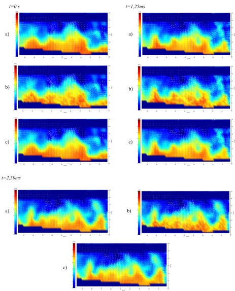
The results of the reconstructions are presented by 2D vector maps of flow velocity with scalar maps (Z component). The measuring plane has been located perpendicular to the main flow, 40 mm behind the plane trailing edge, 10 angle of attack and flow velocity was 5m/s. The flow was captured with the sampling period 1,25ms. The upper part of vector maps corresponds to the location behind the plane trailing edge.

The accuracy of the reconstruction method based on the known correspondences was approximately +/- 1% (for all components) compared with the results from Dynamic Studio.

t=0 s t=1,25ms

t=2,50ms

Figure 6. 2D vector maps of flow velocity with scalar map (Z component) in time t: (a) the reconstruction in paragraph 2., (b) the reconstruction in paragraph 3., (c) Dynamic Studio

a) a)

b)

b) _b)

c) c)

a) b)

4 Conclusion

The paper describes two approaches for evaluation of data obtained by 3D PIV method that can be used in situations where commercial available softwares can fail. The reconstruction based on known correspondence (paragraph 2.) is applicable in cases where the measurement area recorded through objects (eg. cylindrical, convex, concave glass) which significantly distort the images of calibration pattern and satiating particles. The reconstruction by commercial software (eg. Dynamic Studio) often fails in these cases. It was shown that the third order of the polynomial fitting model (paragraph 2.2) is sufficient in most cases. Otherwise it is possible to choose a higher order.

The reconstruction based on intrinsic and extrinsic parameters of cameras (paragraph 3.) is applicable in case where the calibration target can´t be put into the measuring area or where is not possible to move with the calibration target inside the area (eg. long pipe, tunnel). The reconstruction cannot be performed by conventional commercial softwares in such cases. The error in the results is mainly caused by high sensitivity to inaccuracy of the measured parameters (R,t,K).

Acknowledgment

This work was supported by the Ministry of Education, Youth and Sport of the Czech Republic within the SGS project no. 21066/115 on the Technical University of Liberec.

References

1. C. TROPEA, A. L. YARIN, J. F. FOSS: Handbook of experimental fluid mechanics, Volume 1, Springer, 1556 pgs, 2007.

2. L. M. SUÁSTEGUI: Overview on stereoscopic Particle Image Velocimetry, Instituto Politécnico Nacional, Santa Catarina, Mexico, 16 pgs, 2012.

3. J. HOFFMAN, C. JOHNSON, The Mathematical Secret of Flight, Normat 57, 4, pp.1–25, (2009)

4. J. HOFFMAN, C. JOHNSON, Resolution of d’Alembert’s paradox, Journal of Mathematical Fluid Mechanics, Vol.12 (3), pp.321-334, (2010)

5. P. MANNEVILLE, Instabilities, Chaos and Turbulence. Imperial College Press, 2004

6. V. URUBA, On 3D Flow-Structures behind an

Inclined Plate, EFM 2016, Experimental fluid

mechanics. in Mariánské Lázn, 15.11-18.11., Czech Republic, 6p. (2016)

7. M. BSIBSI: Advances in stereoscopic Particle Image Velocimetry and Application to Supersonic Base Flow Exhaust Plume Interaction, TUDelft, 129 pgs, 2004. 8. V. KOPECKÝ: Laser anemometri in fluid Mechanics,

Ed. TRIBUN EU s.r.o., 204 pgs, Brno 2008, in Czech Republic.

9. B. TUROOVÁ. 3D Recnstruction of Scene from Stereo Images, 48 pgs, Charles Univesity in Prague, 2008.

10. J. Y. BOUGUET, Computational Vision [online] Camera Calibration Toolbox for Matlab,2005, URL: