Piecewise linear Wilson lines
Frederik F. Van der Veken1,a
1Department of Physics, University of Antwerp, Groenenborgerlaan 171, 2020 Antwerpen, Belgium
Abstract. Wilson lines, being comparators that render non-local operator products gauge invariant, are ex-tensively used in QCD calculations, especially in small-xcalculations, calculations concerning validation of factorisation schemes and in calculations for constructing or modelling parton density functions. We develop an algorithm to express piecewise path ordered exponentials as path ordered integrals over the separate seg-ments, and apply it on linear segseg-ments, reducing the number of diagrams needed to be calculated. We show how different linear path topologies can be related using their colour structure. This framework allows one to easily switch results between different Wilson line structures, which is especially useful when testing different structures against each other, e.g. when checking universality properties of non-perturbative objects.
1 Introduction
In the so-calledeikonal approximation, a moving quark is considered to emit only soft and collinear radiation, which can be resummed into a Wilson line. One case where we could use the eikonal approximation, is for a quark in a dense medium (see e.g. [1] and [2], where in the latter the medium is reduced into a shockwave).
A Wilson line on a path with endpointsaμandbμ trans-forms as
U(b;a) →ei gα(b)U
(b;a)e−i
gα(a), (1)
which can be utilised to make bilocal operator products gauge-invariant. E.g. in the TMD approach, the opera-tor definition for a transverse momentum dependent par-ton density function contains a bilocal product of quark field operatorsψ(z)ψ(0) [3, 4]. One then inserts a Wilson line (also called agauge linkin this approach) such that the resulting factorψ(z)U(z; 0)ψ(0) is gauge invariant. As the gauge transformation of the Wilson line only depends on its endpoints, there is some freedom on the choice of the path. The correct path will be constructed by eikonal-ising the quark fields and identifying the appropriate gluon radiation [5–7].
Other applications of Wilson lines include the calcu-lation of soft factors [8–11], the study of jet quenching [12], a recast of QCD in loop space where the geometric evolution of rectangular loops can be related to its energy evolution [13–17], etc.
A general Wilson line is an exponential of gauge fields along a pathC, defined as follows:
U =Peig
CdzμAμ(z). (2)
Because the gauge fields are non-Abelian, i.e.Aμ =taAaμ, they have to bepath ordered, denoted by the symbolPin
ae-mail: [email protected]
(2), to avoid ambiguities. The fields are ordered such that the fields first on the path are written leftmost. After mak-ing a Fourier transform the path content is fully described by the following integrals:
In= 1 n! P
dλ1 · · ·dλn
zμ11· · ·zμn
n
e−i
n
ki·zi, (3)
such that then-th order term of the Wilson line expansion is given by
Un=(ig)n
d4k1 (2π)4· · ·
d4kn
(2π)4 Aμn(kn)· · ·Aμ1(k1)In. (4)
2 Piecewise Path Ordered Integrals
We will investigate piecewise functions consisting of M
continuously differentiable segments (in particular, each segment should be defined over an interval that is not a single point). The path-ordered integral over one segment is simply
S2J= aJ+1
aJ
dx1
x1
aJ
dx2 · · ·
xn−1
aJ
dxn fJ(x1)fJ(x2)· · ·fJxn, (5)
Such that we can express the path-integral over the full path in function of the segment integrals as
In= n
i=1 ⎡ ⎢⎢⎢⎢⎢ ⎢⎢⎢⎢⎢ ⎢⎢⎢⎣ ⎛ ⎜⎜⎜⎜⎜ ⎜⎜⎝ i
j=1
Jj−1−1
Jj=i−j+1
⎞ ⎟⎟⎟⎟⎟ ⎟⎟⎠
J0−1=M ⎛ ⎜⎜⎜⎜⎜ ⎜⎜⎜⎜⎜ ⎜⎜⎜⎝
All i
j=1
Slj(Jj)
where
i j=1
lj=n ⎞ ⎟⎟⎟⎟⎟ ⎟⎟⎟⎟⎟ ⎟⎟⎟⎠ ⎤ ⎥⎥⎥⎥⎥ ⎥⎥⎥⎥⎥ ⎥⎥⎥⎦. (6)
E.g. the third order integral is given by
I3=
M
J=1
S3J+ M
J=2
J−1
K=1
SJ1SK2+S2JSK1
+
M
J=3
J−1
K=2
K−1
L=1
S1JS1KSL1,
C
Owned by the authors, published by EDP Sciences, 2015
It is also possible to give a recursive definition:
In(M)= M
J=1
SJn+ M
J=2
n−1
i=1
SJi In−i(J−1). (7)
Eqs. (6) and (7) literally translate to a Wilson line; just replace everyS with anU, for instance:
U3=
M
J=1 UJ
3+2
M
J=2
J−1
K=1 UJ
(1U
K
2)+
M
J=3
J−1
K=2
K−1
L=1 UJ
1U
K
1U
L
1,
where
UJ n =
ig 16π4
n
d4k1 · · ·d4kn Aμ1(k1)· · ·Aμn(kn)S
J n.
The physical interpretation of then-th order formula is a collection of all possible diagrams forn-gluon radiation from aM-segment Wilson line.
Consider now the product of e.g. three Wilson lines, labelled UA, UB and UC. Expanding the exponentials and collecting terms of the same order ingwe get:
UAUBUC=
1+U1A+U1B+UC1
+UA
1U
B
1 +U
A
1U
C
1 +U
B
1U
C
1 +U
A
2 +U
B
2 +U
C
2
+UA
1U1BUC1 +U
A
1U2B+U1AU2C+U
B
1UC2 +U
A
2U1B
+UA
2UC1 +U2BU1C+U3A+U3B+U3C
+. . . ,
which equals, up to third order, the sum of the first, sec-ond and third order full integrals. In other words, we can equate a product of Wilson lines to one Wilson line con-sisting of several segments. The proof easily generalises to all orders. Note that the order of the segments is re-versed w.r.t. the order of the product (because we read the lines from right to left), e.g. the productUAUBUC is a line UCBA, with first segmentC, second segment Band last segmentA.
3 Linear Path Segments
The results from the former section are general results, i.e. valid for any path. Let us now turn our focus towards linear paths only, as these are the most commonly used in literature. For every segment there exist four possible path structures: it can be a finite segment connecting two points, it can be a segment connecting ±∞ and a point
rμ, or it can be a fully infinite line connecting−∞with+∞.
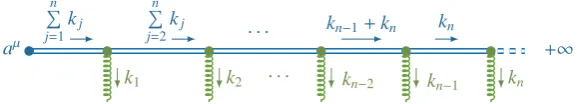
We start by considering a line from a pointaμto+∞, along a direction ˆnμ. Such a path can be parameterised as
zμ=aμ+λnˆμ λ=0. . .∞. (8)
Using (3), it is straightforward to calculate the segment integrals for a lower bound Wilson line:
Il.b.n =nˆμ1· · ·nˆμneia·
j
kj n
j=1 i
ˆ
n·n l=j
kl+iη
. (9)
The iηare convergence terms added to regularise the ex-ponent.We can reconstruct this result using the following Feynman rules:
Propagator: k = i
ˆ
n·k+iη (10a)
External point:
k
aμ =eia·k
(10b)
Line to infinity: +∞ =1 (10c)
Wilson vertex: j i
μ,a
k =ignˆμ(ta)i j (10d)
In order to use this Feynman rules in a consistent way, the momenta of the gluons should always be pointing out-wards, starting from the external point. As an illustration, the resultingn-th order diagram is drawn in figure 1.
Next we investigate a path that starts at−∞and goes up to a pointbμ, which we parameterise as
zμ=bμ+nˆμλ λ=−∞. . .0. (11)
The resulting path integral is almost the same as before:
Inu.b.=nˆμ1· · ·nˆμne
ib·
j
kj n
j=1 −i
ˆ
n· j l=1
kl−iη
(12)
which differs from (9) only in the accumulation of mo-menta in the denominators and the sign of the convergence terms. We can use the same Feynman rules if we keep the convention that gluon momenta are radiated outwards from the external point. Reversing the path flow is the same as taking the Hermitian conjugate of a Wilson line, which is defined for a line from a pointaμto a pointbμas:
U†=Pe−ig
b
a
dz·A
, (13)
where the symbolPdenotes anti-path ordering. To be able to treat all segments on an equal basis, we put the fields in the Hermitian conjugate in non-reversed order by revers-ing the momentum labels. This allows us to relate them to the former results (9) and (12):
U(†+∞;a)=U(a;−∞)nˆ→ −ˆn, (14a)
U(†b;−∞)=U(+∞;b)nˆ→ −ˆn. (14b)
We will indicate the direction of ˆnwith a blue arrow on the Wilson line.
We now introduce a shorthand notation to denote the path structure for a Wilson line segment. The first two structures we calculated before are represented by:
U(+∞;a) N
= , (15a)
U(b;−∞) N
+∞
aμ
k1 n
j=1
kj
k2 n
j=2
kj · · ·
· · · kn−2 kn−1
kn−1+kn
kn kn
Figure 1.n-gluon radiation for a Wilson line going fromaμto+∞.
On the other hand, the two structures with reversed ˆnare then represented by:
U(a;+∞) =U(a;−∞)nˆ→ −ˆn N
= , (16a)
U(−∞;b) =U(+∞;b)nˆ→ −ˆn N
= . (16b)
A nice feature of this notation is that we get a “mirror re-lation”:
†= , †= ,
which is literally the same as (14).
Next we investigate a Wilson line on a finite path, go-ing from a pointaμ to a pointbμ. We parameterise this as:
zμ=aμ+nˆμλ λ=0 . . .b−a. (17) Dropping the factor in front of the integral, we find a re-cursion relation:
Infin(k1,...,kn)=
i ˆ
n·k1
Infin.−1(k1+k2,...,kn)−Infin.−1(k2,...,kn)
(18)
which we can solve exactly by careful inspection (reintro-ducing the factor in front):
Infin.=nˆμ1· · ·nˆμn
n
m=0
m
j=1 i eia·kj
ˆ
n·m l=j
kl n
j=m+1
−i eib·kj
ˆ
n· j l=m+1
kl . (19)
Using the fact that this kind of chained sum can in general be written as a product of two infinite sums:
∞
n=0
n
m=0
AmBn−m= ⎛ ⎜⎜⎜⎜⎜ ⎝
∞
i=0
Ai ⎞ ⎟⎟⎟⎟⎟ ⎠ ⎛ ⎜⎜⎜⎜⎜ ⎜⎝
∞
j=0
Bj ⎞ ⎟⎟⎟⎟⎟ ⎟⎠,
we can transform equation (19) into a product of two Wil-son lines:
U(b;a) =U(†+∞;b)U(+∞;a)=U(b;−∞)U†(a;−∞), (20)
which can be illustrated schematically as:
= ⊗
= ⊗ †.
Finally, the last possible path structure for a linear seg-ment is a fully infinite line, going from−∞to+∞along a direction ˆnμand passing through a pointrμ. Such a path can be parameterised as:
zμ=rμ+nˆμλ λ=−∞. . . +∞. (21)
Naively, one could think thatIinf.
n consists ofn−1 integrals
that evaluate to the Fourier transform of a Heaviside θ -function, and one integral—the outermost—that evaluates to a Diracδ-function. In fact, although this is mathemati-cally not correct because it leads to a divergent expression of theδ-function, one can show by regularising the path as in [18] that this is indeed the result, as long as theδ -function is used in conjunction with the sifting property (and not by its exponential representation). The result is then
Iinf.
n =
n−1
1 i
ˆ
n·n j
kl+iη 2π δ
⎛ ⎜⎜⎜⎜⎜ ⎝nˆ·
n
1
kj+iη ⎞ ⎟⎟⎟⎟⎟
⎠. (22)
We conclude that the correct way to draw an infinite Wil-son line, is to put all radiated gluons on one side from the pointrμ, where the line piece connecting the point to the first gluon is a cut propagator having the following Feyn-man rule:
Cut propagator: k =2π δ(ˆn·k+iη) (23)
4 Relating Different Path Topologies
Not including the infinite line, we can relate the remaining six path structures to each other. If we choose the follow-ing two structures:
=nˆμ1· · ·nˆμneir·
j
kj n
j=1 i
ˆ
n·n l=j
kl+iη
, (24a)
=nˆμ1· · ·nˆμneir·
jkj
n
j=1 −i
ˆ
n· j l=1
kl+iη
, (24b)
we can express the remaining four in function of them:
= ˆn→−ˆn, (25a)
=
ˆ
n→−ˆn, (25b)
= ⊗ , (25c)
= ⊗ nˆ→−ˆn. (25d)
The two first structures aren’t fully independent either, as they are related by a sign difference and an interchange of momentum indices:
= (−)n
(k1,...,kn)→(kn,...,k1)
We can exploit this relation when connecting a Wilson line to a blob. This blob can be constructed from any com-bination of Feynman diagrams, but cannot contain other Wilson lines.1 For the structure given in (24a) this is:
. . .
F
= (ig)ntan· · ·ta1
Dk Il.b.n Fa1···an
μ1···μn(k1, . . . ,kn),
where we absorbed the gluon propagators into the blob
Fa1···an
μ1···μn. Furthermore, we always define the blob as the
sum of all possible crossings; it is thus symmetric under the simultaneous interchange of Lorentz, colour, and mo-mentum indices. Because every Lorentz index ofFis con-tracted with the same vector ˆnμ, it is automatically sym-metric in these. These two symmetries imply that an change of momentum variables is equivalent to an inter-change of the corresponding colour indices. In particular, it is now straightforward to relate (24b) to (24a):
. . .
F
= (−ig)ntan· · ·ta1
Dk Inl.b.Fμ1···an···aμ1n(k1, . . . ,kn).
Often the blob has a factorable colour structure, i.e.
Fa1···an
μ1···μn(k1, . . . ,kn)=C
a1···anF
μ1···μn(k1, . . . ,kn). (27)
If we now define the following notations:
C=tan· · ·ta1Ca1···an, C=tan· · ·ta1Can···a1, (28a)
we can simply write
. . .
F
= C . . .
F
, (29a)
. . .
F
= (−)nC . . . F
. (29b)
The yellow, ‘photon-like’ wavy lines are just a reminder that there is no colour structure left in the blob. For a fac-torable blob example, take e.g. the three gluon vertex:
F =gfa1a2a3(k
1−k2)ρDμ1ν(k1)Dμν2(k2)Dρμ3(k3)+cross.
,
with colour structure fa1a2a3. This implies thatC=−C:
= .
Of course, a lot of blob structures won’t be colour torable, but we can always write these as a sum of fac-torable terms:
Fa1···an
μ1···μn(k1, . . . ,kn)=
i Ca1···an
i Fiμ1···μn(k1, . . . ,kn),
1If one is interested in interactions between different Wilson lines, it
is sufficient to treat the different lines as different segments of one line (as is explained in the end of section 2).
such that we can repeat the same procedure as before
. . .
F
=
i
Ci . . .
Fi
, (30a)
. . .
F
= (−)n
i
Ci . . .
Fi
. (30b)
5 Piecewise Linear Wilson Lines
When connecting a n-gluon blob to a piecewise Wilson line, the n gluons aren’t necessarily all connected to the same segment, but the n-gluons can be divided among several segments; this is the physical interpretation of for-mula (6). Because the blob is summed over all crossings, multiple-segment terms can be related by straightforward substitution, e.g.
UJ
1U
K
2 =U
J
2U
K
1(r
J↔rK,nJ↔nK)
, (31)
etc. When connecting e.g. a 4-gluon blob, we need to cal-culate exactly 5 diagrams, independent on the number of segmentsM. These diagrams are (cf. (6)):
UJ
4,U
J
3U
K
1,U
J
2U
K
2,U
J
2U
K
1U
L
1,andU
J
1U
K
1U
L
1U
O
1.
They are the easiest represented schematically:
F F F
F F
(32) Now what about the different path structures, as de-fined in (24)? We can use the same trick as in the end of the former section, viz. a sign change and an interchange of the corresponding colour indices. For instance:
F
= (−)2
Fa 3↔a4
.
The easiest way to implement this, is to define a path func-tionΦper diagram for a given blob, that gives the colour structure in function of the path type. For the leading order 2 gluon blob, this is straightforward:
: Φ(J)=CF, (33a)
whereφJrepresents the structure of the segment:
φJ=⎧⎪⎪⎨⎪⎪⎩
0 J=
1 J= (34)
Keep in mind that in our original definition of the Wilson line (2), colour indices are not yet traced, hence equations (33) should still be multiplied with an unit matrix1. Sim-ilarly for the leading order 3-gluon blob we find:
: Φ(J)=−iN
2CF, (35a)
: Φ(J,K)=−i (−)φJ+φKN
2CF, (35b)
: Φ(. . .)=−i (−)φJ+φK+φLN
2CF.(35c)
For non-factorable blobs we use the same trick as in (30), by givingΦan extra index to identify the sub diagram it belongs to.
Let us introduce a new notation, to indicate a full di-agram, but without the colour content, in which a blob is connected tomWilson line segments, withnigluons
con-nected to thei-th segment:
WJm···J1
nm···n1, (36)
where we will write the indices from right to left for con-venience. Returning to the 4-gluon blob, we can now write the full result for a factorable blob using (6):
U4=
M
J
Φ4WJ
4+
M
J=2
J−1
K=1
Φ3 1WJK
3 1 + Φ2 2W
JK
2 2
+
M
J=3
J−1
K=2
K−1
L=1
Φ2 1 1WJKL
2 1 1
+
M
J=4
J−1
K=3
K−1
L=2
L−1
O=1
Φ1 1 1 1WJKLO
1 1 1 1 +symm., (37)
where the symmetrised diagramsΦ1 3W1 3JK,Φ1 2 1W1 2 1JKL, andΦ1 1 2WJKL
1 1 2 are calculated using (31), interchanging also theφJ. For a non-factorable blob, every term is just
replaced by a sum over sub diagrams. It is important to realise that both theΦni···andWni···can be calculated
in-dependent of the path structure, giving a result depending onnJ,rJandφJ.
So far we have only calculated amplitudes. To get probabilities from these, we can do this in the standard way, viz. squaring diagrams and combining them order by order (squared terms and interference terms), or we could treat the squared diagram as one Wilson line, where the segments to the right of the cut are the hermitian conju-gate of those to the left . We choose to continue with the latter case, where we now have three distinct sectors of diagrams: a sector where the blob is only connecting seg-ments left of the cut, a sector where the blob is only con-necting segments right of the cut, and a sector where the
blob is connecting segments both left and right of the cut. In other words:
U=Uleft+Ucut+Uright. (38)
For the first two nothing changes, the calculations go as before. For the example of the 4-gluon blob, the first sec-torU4
leftis almost exactly equal to (37), but the sums run up only toMc, the number of segments before the cut,
in-stead ofM. The last sectorU4
rightis simply the hermitian conjugate of this, starting at Mc+1. For the remaining sectorWcutwe need to define a cut blob. Given a blob, several possible cut blobs might exist, depending on the number of gluons to the left and right of the cut. E.g. the leading order 4-gluon cut blobs are given by
= +cross., (39a)
= + +cross., (39b)
where the crossings are to be made on the sides of the cut separately. Also note that when the cut blob is more com-plex, it should be summed over all possible cut locations. Consider e.g. the fermionic part of the NLO 2-gluon cut blob:
= + + . (40)
Returning to the sector Wcut, we investigate which dia-grams are added in comparison to (32) due to the cut. First note that a Wilson line segment is never cut itself by its nature, so cuts are always placedbetweentwo segments.2 Another remark is that we cannot simply use relation (31) as before, because it could change the cut topology. Cut diagrams are sorted depending on how its gluons are dis-tributed on the left resp. right side of the cut, and con-nected to the appropriate cut blob. For instance the second diagram of (32), W4
3 1 can be cut in one way only, con-necting the Wilson line to cut blob (39a), but the fourth diagram, W4
2 1 1, can be cut in two ways: cutting with one gluon on the left (written asW4
2 1|1 and connected to (39a)), or cutting with two gluons (written asW2|1 14 and connected to (39b)). Other cut topologies can be related by Hermitian conjugation when switching left and right sides, e.g.W1 1|2JKL =W2|1 1†LK J. In case of the 4-gluon blob,
2There seem to exist exceptions to this in existing literature, but it is
the following diagrams have to be added to (32):
(41)
Now we have the necessary ingredients to write the cut sector for the 4-gluon blob:
W4 cut=
M
Mc+1
Mc
1
WJK
3|1 +h.c.
+WJK
2|2
+
M
Mc+2
J−1
Mc+1
Mc
1
WJKL
2 1|1+symm.
+WJKL
2|1 1
+
M
Mc+2
J−1
Mc+1
Mc
2
L−1
1
WJKLO
1 1|1 1
+
M
Mc+3
J−1
Mc+2
K−1
Mc+1
Mc
1
WJKLO
1 1 1|1+h.c. (42)
6 Example Calculation
Let us recapitulate our framework with a small example; we will calculate the 2-gluon blob connected to a general Wilson line at NLO. At any order, there are 3 possible 2-gluon diagrams:
(43) At NLO the blob is just a LO gluon propagator (here given in Feynman gauge):
F=−i (2π)4δ(k1+k2)δab 1
k2 1+iε
gμ1μ2, (44)
and the cut blob just a radiated gluon integrated over:
F =−(2π)5δ(k1+k2)δabθk1+ δ
k21gμν. (45)
The colour factors (for both) are given by (33). The first di-agram is then given by, using dimensional regularisation:
WJ
2 =−ig
2CFμ2nˆ2
J
dωk
(2π)ω 1 ˆ
nJ·k+iη
1 iη
1
k2 1+iε
(46)
=−1
2αsCF ⎛
⎜⎜⎜⎜⎝1+ln 4πμ2nˆ 2
J η2 ⎞
⎟⎟⎟⎟⎠ (47)
Acknowledgements
I am very grateful to the organisers of the Transver-sity 2014 conference for creating such a fruitful environ-ment. Furthermore I would like to thank I.O. Chered-nikov, M. Echevarria, L. Gamberg, A. Idilbi, T. Mertens, A. Prokudin and P. Taels for useful discussions and in-sights.
References
[1] J.P. Blaizot, F. Dominguez, E. Iancu, Y. Mehtar-Tani, JHEP1301, 143 (2013),1209.4585
[2] E. Iancu, J. Laidet, Nucl.Phys. A916, 48 (2013),
1305.5926
[3] J. Collins,Foundations of perturbative QCD, Vol. 32 ofCambridge monographs on particle physics, nu-clear physics and cosmology(Cambridge University Press, Cambridge, 2011)
[4] M.G. Echevarría, A. Idilbi, I. Scimemi, Phys.Lett. B726, 795 (2013),1211.1947
[5] A.V. Belitsky, X. Ji, F. Yuan, Nucl.Phys.B656, 165 (2003),hep-ph/0208038
[6] D. Boer, P. Mulders, F. Pijlman, Nucl.Phys. B667, 201 (2003),hep-ph/0303034
[7] I. Cherednikov, N. Stefanis, Nucl.Phys.B802, 146 (2008),0802.2821
[8] M.G. Echevarria, A. Idilbi, I. Scimemi, JHEP1207, 002 (2012),1111.4996
[9] T. Becher, G. Bell, S. Marti, JHEP1204, 034 (2012),
1201.5572
[10] A. Idilbi, T. Mehen, Phys.Rev.D75, 114017 (2007),
hep-ph/0702022
[11] J.y. Chiu, A. Fuhrer, A.H. Hoang, R. Kelley, A.V. Manohar, Phys.Rev. D79, 053007 (2009),
0901.1332
[12] I. Cherednikov, J. Lauwers, P. Taels, Eur.Phys.J. C74, 2721 (2014),1307.5518
[13] I. Cherednikov, T. Mertens, Phys.Lett. B734, 198 (2014),1404.6713
[14] I. Cherednikov, T. Mertens, F. Van der Veken, Phys.Part.Nucl.44, 250 (2013),1210.1767
[15] F.F. Van der Veken, PoSHadron2013, 134 (2013),
1405.4017
[16] T. Mertens, EPJ Web Conf.73, 02011 (2014) [17] T. Mertens, PoSHadron2013, 135 (2013) [18] P. Kotko, JHEP1407, 128 (2014),1403.4824 [19] M.G. Echevarria, A. Idilbi, I. Scimemi,
Int.J.Mod.Phys.Conf.Ser. 25, 1460005 (2014),
1310.8541
[20] M.G. Echevarria, A. Idilbi, I. Scimemi, Phys.Rev. D90, 014003 (2014),1402.0869