Very Fast Current Diagnostic for Linear Pulsed Beams

* _{Corresponding author: [email protected]}

Very Fast Current Diagnostic for Linear Pulsed Beams

Vincenzo Nassisi*_{, Domenico Delle Side and Vito Turco}

Dipartimento di Matematica e Fisica, Lab. LEAS – Università del Salento and I.N.F.N. sect. of Lecce, Italy

Abstract. Fast current pulses manage lasers and particle accelerators and require sophisticate systems to be detected. At today Rogowski coils are well known. They are designed and built with a toroidal structure. In recently application, flat transmission lines are imploded and for this reason we develop a linear Rogowski coil to detect current pulses inside flat conductors. To get deep information from the system, it was approached by means of the theory of the transmission lines. The coil we build presents a resistance but it doesn’t influence the rise time of the response, instead the integrating time. We also studied the influence of the magnetic properties of coil support. The new device was able to record pulses of more hundred nanoseconds depending on the inductance, load impedance and resistance of the coil. Furthermore, its response was characterized by a sub-nanosecond rise time (~100 ps), The attenuation coefficient depends mainly on the turn number of the coil, while the quality of the response depends both on the manufacture quality of the coil and on the magnetic core characteristics. In biophysical applications often, a double line is employed in order to have a sample as control and a sample stressed by a light source. So, in this case we build two equal plane lines by 100 Ω characteristic resistance connected in parallel. We diagnosed the current present in a line. The attenuation factor resulted to be 11,5 A/V.

1 Introduction

Rogowski coil is a well-known electric current detector since about a century[1]. Nevertheless, today its capabilities are still of great interest. TEA lasers and accelerator system need to detect fast current[2]. Also flat transmission lines utilised for radiofrequency biophysical experiments[3] need to control the current.

It was developed to detect variable currents fluxing in a conductor, which is responsible of the magnetic field around the conductor proper axis. In principle, the voltage provided by the coil is proportional to the input pulse current derivative and in order to obtain a sound measure of the originating signal, an integrating circuit is applied[4]. For high frequency signals, its response becomes self-integrating, providing an attenuation factor independent of the time duration or signal frequency. Moreover, the behaviour of the system is more complex for fast pulses due to the creating a capacitance with the metallic shield.

In the past, this detail has been analysed and developed by a few authors [5-7]. Under a few restrictions, the proposed device allows to justify its behaviour for fast pulses, large dimensions of the detector and manufacture quality.

To study our detector, we build two equal plane lines by 100 Ω characteristic resistance connected in parallel. We diagnosed the current present in a line.

2 Theory

The theory of the Rogowski coil is based on the main laws of electromagnetism.

2.1. Rogowski Coil

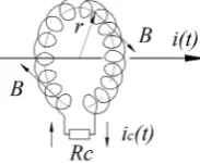
A current fluxing in a conductor generates a magnetic field dependent on distance 𝑟𝑟 from it and a toroidal inductor is influenced by the magnetic flux derivative.

Fig. 1 shows a sketch of the system.

Fig. 1: Electrical circuit of a toroidal Rogowski coil with the input current in the centre.

Applying the Kirchhoff’s equation [1, 8, 9], in the Laplace domain we have,

𝑝𝑝𝐼𝐼

$

(𝑝𝑝)

'₎(

= 𝑝𝑝𝐿𝐿

,

𝐼𝐼(𝑝𝑝) + 𝑅𝑅

,

𝐼𝐼(𝑝𝑝)

(1) with 𝐼𝐼$(𝑝𝑝) and 𝐼𝐼(𝑝𝑝) are the Laplace transforms of the input

𝐿𝐿,= 𝜇𝜇2𝑛𝑛4𝐴𝐴 2𝜋𝜋𝜋𝜋 is the inductance of the coil, 𝑛𝑛 is the number of loops and 𝑝𝑝 is the Laplace variable. Now, hypothesizing a Heaviside function as current signal, i.e.

𝑖𝑖(𝑡𝑡) = 𝐼𝐼2𝑢𝑢(𝑡𝑡), its transform is 𝐼𝐼$(𝑝𝑝) = 𝐼𝐼2 𝑝𝑝. Then the real output current results

𝑖𝑖

,

(𝑡𝑡) =

9₎:

𝑒𝑒

<

=

>

∙ 𝑢𝑢(𝑡𝑡)

(2) where 𝜏𝜏 = 𝐿𝐿, 𝑅𝑅,. This shows that the overall attenuation obtained in the detector with respect to the input current strongly depends on time due to the exponential factor. If we consider an observation time 𝑇𝑇 ≪ 𝜏𝜏 (more in general,

𝑇𝑇 is the pulse length of the input pulse), then the response on resistive load becomes

𝑖𝑖

,

(𝑡𝑡) =

9₎:

∙ 𝑢𝑢(𝑡𝑡)

(3) The above result implies that the detector is also able to detect high frequency currents. Indeed, the steady-state response can be obtained from Eq. 1 substituting 𝑝𝑝

with 𝑗𝑗𝑗𝑗, where 𝑗𝑗 is the imaginary unit and 𝑗𝑗 the frequency of the input current. The attenuation factor is

$((J)

$(J)

=

K )

LM

LMNO(_P( (4)

then, to get a frequency independent response, in the steady-state case we observe that the attenuation is constant if 𝑅𝑅, 𝐿𝐿, ≪ 𝑗𝑗.

We stress that the results obtained do not depend on the shape of the coil loops neither on the area of each turn. Indeed, such assumptions are not satisfactory for short pulses.

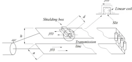
The Rogowski coil we developed is devote for planar currents. This model is very useful, apart for laser discharges, also plane transmission lines. This last allows us to perform experiments of radiofrequency biophysical stresses [7, 9-11]. A sketch of a planar current is shown in Fig. 2. A current 𝑖𝑖(𝑡𝑡) in the conductor (width 𝑎𝑎) determines a current density that we call 𝑗𝑗 𝑡𝑡 = 𝑖𝑖(𝑡𝑡) 𝑎𝑎.

Fig. 2: Sketch of a Rogowski coil employed in a planar conductor.

Again, applying the Kirchhoff’s equation, in the Laplace domain we have

𝑝𝑝𝐼𝐼

$

𝑝𝑝

₄₎'(R_S

= 𝑝𝑝𝐿𝐿

,

𝐼𝐼 𝑝𝑝 + 𝑅𝑅

,

𝐼𝐼 𝑝𝑝

(5)

where 𝑑𝑑 is coil length and again 𝐼𝐼$(𝑝𝑝) is the Laplace transform of the input current 𝑖𝑖(𝑡𝑡).

For an Heaviside-like input current, the corresponding Laplace transform is 𝐼𝐼$(𝑝𝑝) = 𝐼𝐼2 𝑝𝑝, and the final form of Eq. 5 becomes

𝐼𝐼

2₄₎'(R_S

= 𝑝𝑝𝐿𝐿

,

𝐼𝐼 𝑝𝑝 + 𝑅𝑅

,

𝐼𝐼 𝑝𝑝

(6)

whose real solution is

𝑖𝑖

,

𝑡𝑡 =

₎KR_S

𝐼𝐼

2

𝑒𝑒

<

O(

P(J

₍₇₎

and for 𝑡𝑡 ≪ 𝐿𝐿, 𝑅𝑅,, the response will be time independent:

𝑖𝑖

,

(𝑡𝑡) =

₎KR_S

𝐼𝐼

2

(8)

This result is comparable to that obtained for the toroidal Rogowski coil described by Eq. 3, apart from the correction factor 𝑑𝑑 2𝑎𝑎. Again, utilizing 𝑗𝑗𝑗𝑗 instead of 𝑝𝑝 it is possible to get the steady-state response.

2.2 Rogowski

coil as distributed elements

For fast pulses the above circuits are insufficient because they are unsuitable for transmit fast signals. So we consider the Rogowski coil as composed by distributed elements. It allows us to justify the presence of anomalies on the signal response generally due to imperfect manufacture.

To avoid interferences of stray signals, the coil is enclosed in a shielding box. It is a cracked metallic box operated on the ground conductor. The crack is realized by operating a slim slit on the conductor. The slit changes the current direction which wraps the coil, inducting again the same electromotive force, see Fig. 3.

Fig. 3: Sketch of a flat transmission line with a linear Rogowski coil closed in the shielding box.

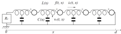
So, to study it, let us to call 𝑓𝑓(𝑡𝑡, 𝑥𝑥) the electromotive force per unit length. Now, the presence of the metallic box exhibits a distributed capacitance along the coil. Let us to call 𝐶𝐶(𝑥𝑥) the capacitance per unit length. Even the inductance of the coil is distributed along the device and per unit length, it is 𝐿𝐿(𝑥𝑥), as well as that of the ground conductor, namely 𝐿𝐿Y(𝑥𝑥). Therefore, the device we analyse can be considered exactly as a transmission line, Fig 4.

Let us consider the electric circuit of this line by means of an infinite number of cells. A typical cell is illustrated in Fig. 4 where 𝑓𝑓(𝑡𝑡, 𝑥𝑥), 𝐿𝐿(𝑥𝑥) and 𝐶𝐶(𝑥𝑥) are the voltage, the inductance and the capacitance per unit length, respectively. Besides, 𝐿𝐿Y(𝑥𝑥), 𝑅𝑅(𝑥𝑥) and 𝐺𝐺(𝑥𝑥) are the inductance of the box conductors, the resistance of the coil wire and the conductance of the insulator per unit length, respectively.

Fig. 4: Electric sketch of a Rogowski coil closed into the

metallic box.

Then, applying Kirchhoff’s equations, the differential of voltage and current for every cell to differential of position depend through the following equations:

[\((J,])

[]

= − 𝑍𝑍 𝑡𝑡, 𝑥𝑥 𝑖𝑖

,

𝑡𝑡, 𝑥𝑥 − 𝑓𝑓(𝑡𝑡, 𝑥𝑥)

(9)

[$((J,])

[]

= − 𝑌𝑌 𝑡𝑡, 𝑥𝑥 𝑣𝑣

,

𝑡𝑡, 𝑥𝑥

with 𝑍𝑍 𝑡𝑡, 𝑥𝑥 and 𝑌𝑌 𝑡𝑡, 𝑥𝑥 the impedance and admittance operators of the circuit per unit length. They correspond to 𝑍𝑍 = 𝑅𝑅 + 𝐿𝐿_RJR + 𝐿𝐿Y_RJR and 𝑌𝑌 = 𝐺𝐺 + 𝐶𝐶 𝑑𝑑𝑡𝑡 . Next, to simplify the solution, the resistance 𝑅𝑅, the inductance 𝐿𝐿Y and the conductance 𝐺𝐺 are neglected and the line is represented by the circuit of Fig. 5. Operating the Laplace transform of Eq. 9, the impedance operator becomes 𝑍𝑍 𝑝𝑝 = 𝑝𝑝𝐿𝐿(𝑥𝑥), the admittance one becomes 𝑌𝑌(𝑝𝑝) = 𝑝𝑝𝐶𝐶(𝑥𝑥) and the electromotive force one becomes 𝐹𝐹 𝑝𝑝, 𝑥𝑥 = 𝑝𝑝𝐼𝐼$(𝑝𝑝)𝐿𝐿𝑑𝑑 𝑛𝑛𝑛𝑛.

Fig. 5: Electric circuit of the Rogowski coil closed inside the metallic box. The voltage and the current along the coil are 𝑣𝑣, 𝑡𝑡, 𝑥𝑥 and 𝑖𝑖, 𝑡𝑡, 𝑥𝑥 , respectively.

Theoretically, the last three parameters should be

x-independent and this depends on the coil manufacture quality. Therefore, under the above constraints, the Laplace transform of Eq. 9 is:

𝑉𝑉

,

𝑥𝑥, 𝑝𝑝 =

_{f' g}e f g_(Ng(gh_h

∙

i

j>hkl_<ij>hk mnjl

KNoijm>hkn

(

10a

)

𝐼𝐼

,

𝑥𝑥, 𝑝𝑝 =

_{f' (g}e f g_(Ng(_h) i

j>hkl_Nij>hk mnjl

KNoijm>hkn

−

e f_f' (10b)

where we have considered the line short-circuited at 𝑥𝑥 = 𝑑𝑑 and closed on resistive load 𝑅𝑅, at 𝑥𝑥 = 0. The parameter 𝜗𝜗 represents the reflection coefficient, namely (𝑅𝑅,− 𝑅𝑅2) (𝑅𝑅,+ 𝑅𝑅2), where 𝑅𝑅2 is the characteristic resistance of the line whose expression is 𝑅𝑅2=

𝑍𝑍(𝑝𝑝) 𝑌𝑌(𝑝𝑝), while the propagation function per unit length is −𝜏𝜏r. In our conditions, the latter is a constant, 𝜏𝜏r= 𝑍𝑍 𝑝𝑝 𝑌𝑌(𝑝𝑝) = 𝐿𝐿𝐶𝐶 and it expresses the delay per unit length. Because it is known to be of the order of 10<t 𝑠𝑠 𝑚𝑚 let us suppose that 𝜗𝜗𝑒𝑒<4whfR _{< 1} and we can

operate the expansion

𝜗𝜗𝑒𝑒

<4whfR

≅ 1 −

𝜗𝜗𝑒𝑒

<4whfR

+𝜗𝜗

4

𝑒𝑒

<zwhfR

−𝜗𝜗

{

𝑒𝑒

<|whfR

+ ⋯

₍₁₁₎ Substituting the Eq. 11 in the first Eq. 10, the voltage across 𝑅𝑅, is obtained placing 𝑥𝑥 = 0

𝑉𝑉

,

𝑥𝑥, 𝑝𝑝 =

_{f' g}e f g_(Ng(g_hh

1 − 𝜗𝜗

~

𝑒𝑒

<4whfR

+

𝜗𝜗𝜗𝜗

~

𝑒𝑒

<zwhfR

− 𝜗𝜗

4

𝜗𝜗

~

𝑒𝑒

<|whfR

∙∙∙

(12) with 𝜗𝜗~= 1 + 𝜗𝜗 = 2𝑅𝑅, 𝑅𝑅,+ 𝑅𝑅r . Instead, substituting the Eq. 11 in the second Eq. 10, the current in 𝑅𝑅, is obtained again placing 𝑥𝑥 = 0

𝐼𝐼

,

0, 𝑝𝑝 =

_{f' g}e f g_(Ng(_h

1 + 𝜗𝜗

9

𝑒𝑒

<4whfR

−

𝜗𝜗𝜗𝜗

9

𝑒𝑒

<zwhfR

+ 𝜗𝜗

4

𝜗𝜗

9

𝑒𝑒

<|whfR

… −

e f_f'

(13) with 𝜗𝜗9= 1 − 𝜗𝜗 = 2𝑅𝑅r 𝑅𝑅,+ 𝑅𝑅r .

For an Heaviside-like input current, the corresponding electromotive force per unit length is constant

𝐹𝐹 𝑝𝑝 =

9h' )

R

S

(14) Using Eq. 14, for 𝑅𝑅,= 𝑅𝑅r, we have 𝜗𝜗 = 0, and consequently 𝜗𝜗~= 1 as well as 𝜗𝜗9= 1. The response at 𝑥𝑥 = 0 becomes:

𝑉𝑉

,

0, 𝑝𝑝 =

9_4f)hghR_S

∙ 1 − 𝑒𝑒

<4whfR

(15a)

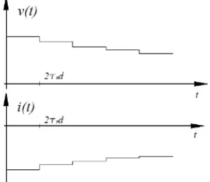
Fig. 6: Pictorial representation of the response waveforms for voltage and current with 𝑥𝑥 = 0 and 𝑅𝑅,= 𝑅𝑅r.

In the time domain, the result is a voltage and current pulse 2𝜏𝜏r𝑑𝑑 long that corresponds to the time of a signal to propagate and came back for the whole line, Fig. 6. Nevertheless, this response does not match the input signal we want to detect. Instead, closing the Rogowski coil on a load resistor of low value such that 𝑅𝑅, < 𝑅𝑅r, it results that −1 < 𝜗𝜗 < 0, 0 < 𝜗𝜗~< 1 and 1 < 𝜗𝜗9< 2. At 𝑥𝑥 = 0 the response is a voltage signal that decreases every 2𝜏𝜏r𝑑𝑑 seconds of a little quantity, while the current signal is initially negative with the overlapping of a small positive signal every 2𝜏𝜏r𝑑𝑑 seconds. Fig.7 shows a pictorial representation of the situation.

Fig. 10: Pictorial representation of the waveforms for voltage and current with 𝑥𝑥 = 0 and 𝑅𝑅,< 𝑅𝑅r.

This result is very interesting particularly if 𝑅𝑅,≪ 𝑅𝑅r because we can have: 𝜗𝜗 ≅ −1, 𝜗𝜗~≅ 0 and 𝜗𝜗9≅ 2 and by the Eqs. 12 and 13 the response is approximately:

𝑉𝑉, 0, 𝑝𝑝 ≅9h_f)g(R_S (16a)

𝐼𝐼,

0, 𝑝𝑝 ≅ −

9h

f) R

S

(16b) Performing the inverse transformation in order to get the time dependent relations, the results are:

𝑣𝑣

g,

(𝑡𝑡) ≅

9h₎g(R_S

𝑢𝑢(𝑡𝑡)

(17a)

𝑖𝑖

g,

(𝑡𝑡) ≅

9₎hR_S

𝑢𝑢(𝑡𝑡)

(17b)

The relations obtained show that the theory developed give results very similar to the one expressed by Eq. 8 but now they deliver more information. Indeed, if the coil is not uniformly shaped, a different electromotive force will be induced at different positions and different values of inductance and capacitance are exhibited. In this case the propagation function per unit length isn’t constant and an overlapped signal propagate along the line generating ripples on 𝑅𝑅,. To attenuate the ripple, authors have suggested to apply some resistors along the coil in order to damp these undesirable signals [13]. In this case, the behaviour of the system improves but the value of the integrating time, that theoretically is 𝐿𝐿𝑑𝑑 𝑅𝑅,, decreases. However, the insertion of the resistors must be realized without creating new loops and/or modify the capacitance values because they could introduce new elements that should modify the behaviour.

2.3

Influence of the coil resistance

During the development of the previous theory, the resistance of the coil wire has been neglected. The response of the Rogowski coil for a Heaviside-like signal is principally characterised by an attenuation coefficient and by a damping time. Then, considering a no-null value for 𝑅𝑅, the voltage on the load 𝑅𝑅, becomes

𝑉𝑉

,

𝑥𝑥, 𝑝𝑝 =

𝐹𝐹 𝑝𝑝 𝑅𝑅

,

𝑝𝑝𝐿𝐿 + 𝑅𝑅 1 + 𝑅𝑅

,

𝑝𝑝𝐿𝐿 + 𝑅𝑅 𝑝𝑝𝜏𝜏

r

1 + 𝑅𝑅

_{𝐿𝐿𝑝𝑝}

ij>kl

K<€jO(>k_€ÅO(>kijm>kn

−

iÅ>kl_ijm>kn

K<€jO(>k_€ÅO(>kijm>kn

(18)

where the parameter 𝜏𝜏 = 𝜏𝜏r 1 + 𝑅𝑅 𝑝𝑝𝐿𝐿. Then, before operating the inverse transformation, it is interesting to note that the part of Eq. 18 in square brackets governs the propagation of the signal. If we consider again the load resistance 𝑅𝑅,~0, condition necessary to get easily the result we expect, at 𝑥𝑥 = 0 the value of this part is 1. Instead, the first part governs the attenuation factor. The inverse transformation of only this first part is very difficult, but the solution can be reached imposing that the coil resistance is generally small. Then, the expansion of the square root, considering only the first two terms is

1 +_{' f}g ≅ 1 + 𝑅𝑅 2𝐿𝐿𝑝𝑝 and Eq. 18 then reads

𝑉𝑉

,

0, 𝑝𝑝 ≅

_{f'Ng KN}e f gO( (

kPÅOfwh KNmPkO

(19)

Always for a Heaviside current signal as input, we have

𝑉𝑉

,

0, 𝑝𝑝 ≅

_{) f'Ng KN}'9hO(g(

kPÅOfwh KNmPkO

transformation, the real voltage on 𝑅𝑅, exhibits an exponential behaviour, namely:

𝑣𝑣

g,

𝑡𝑡 =

_)('Ng9h'g₍(_wh)

𝑒𝑒

<

O=(mPÅO(>h) mP(PÅO(>h) R

S

∙ 𝑢𝑢(𝑡𝑡)

(21)

which for 𝑅𝑅,~0 becomes

𝑣𝑣

g,

𝑡𝑡 ≅

9h₎g(R_S

𝑒𝑒

<

O

PJ

∙ 𝑢𝑢(𝑡𝑡)

(22) Comparing the Eq. 21 to Eqs. 17, we observe that a non-negligible 𝑅𝑅 does not affect the attenuation coefficient but changes only the time behaviour. Therefore, during the design of a Rogowski coil, for high-precision measurements, it is necessary to consider both the values of 𝑅𝑅 and 𝑅𝑅, in order to find the current, while the voltage is still simply the current multiplied by only 𝑅𝑅,.

2.4 Influence of core characteristics

Utilizing magnetic materials for the core of the coil its inductance changes as well as the electromotive force. An inductor with a core having only the real component of permeability, 𝜇𝜇ƒ, larger than 1, has a 𝜇𝜇ƒ times increased inductance value, but also the electromotive force increases of the same factor 𝜇𝜇ƒ. This behaviour could be considered as an advantage, since it reduces the effect of construction anomalies. In fact, loops of different cross section but with the same magnetic properties by constant diameter exhibit very near inductance values. Nevertheless, the use of a magnetic core involves a constant value of the permeability coefficient and of magnetic flux. In this way, a linear response is ensured.

In principle, the time response is not influenced by the permeability 𝜇𝜇ƒ, provided that the latter is constant. Instead, if the permeability has also an imaginary component, the risetime response is increased limiting the applications on frequency range, particularly the maximum frequency value.

3 Experimental Material and method

3.1Material

The device presented in the above sections has been designed and built for recording fast currents fluxing in a plane line. It is made by a Cu wire wound along a Lucide rod of 4 mm diameter 27 mm long. The wire has a

0.11 𝑚𝑚𝑚𝑚 in diameter which provides a maximum value

of turn density of 80 𝑟𝑟𝑟𝑟𝑟𝑟𝑟𝑟𝑟𝑟/𝑐𝑐𝑚𝑚 with a total of 216 turns. The coil load 𝑅𝑅ˆ was the characteristic impedance of a 50 Ω cable, while the value of 𝑅𝑅 has been measured to be of 4 Ω.

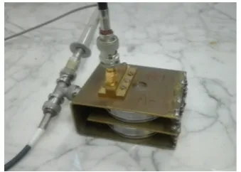
Fig. 11: Double plane transmission line with the linear Rogowski probe on the ground conductor. The transverse dimension is 6 cm.

The transmission line we used in this work was a double transmission line of 100 Ω characteristic impedance connected in parallel as can be seen in Fig. 11. Both the lines are composed by two plane Cu conductors 6 cm wide, spaced 2 cm. The end of each line is closed on a resistive load by means of 4 parallel resistors of 400 Ω, equal distributed. Similar configurations are present in the laser system MOPA and in biophysical applications.

Under this configuration, the current in each line is the half of the total current and Eq. 22 is modified in

𝑣𝑣

g,

𝑡𝑡 ≅

9h₄₎g(R_S

𝑒𝑒

<

O

PJ

∙ 𝑢𝑢 𝑡𝑡

(23) In practice the expression (23) might contain the value of 𝑅𝑅, and, being the value of 𝐿𝐿 of the order of 500 𝑟𝑟𝑛𝑛, the time duration of the signals we can record may be of at max 200 𝑟𝑟𝑟𝑟.

The Rogowski coil is applied on the ground conductor of the plane transmission line. The slit operated in correspondence of the coil was 35 mm long in order to guide the input current around the coil.

3.2Results

Fig. 12: Sketch of the electric circuit used to calibrate the linear probe.

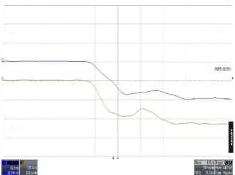
Fig. 13: Waveform of the input and output signals. Upper lower is the input current; upper trace is the output signal. Time scale 50 ns/div.

The waveform response is very near to the input one, as can be seen in Fig 13, where we have used one pulse forming line of 16 m.

The lower trace scale is 1 V/div which correspond to

1 V×_çrŽz| K₄= 0.46 A/div, while the upper trace is 50 mV/div while correspond to 50 mV div . The attenuation factor is about 12 𝐴𝐴/𝑉𝑉, while theoretically one expect 216× |r_4•× _çrK = 9.6 A/V.

The discrepancy we found is mainly due to the distributed current inside the line owing to the slit that we have operate only for 50 mm. The maximum time duration of the detection signal is about 157 ns, as can be seen in Fig. 13.

In order to test the behaviour of our device, we perform an experiment with very short pulse utilising as pulse forming line of about 5 cm. The result of the latter test are illustrated in Fig. 14, where the time scale is 1 ns/div.

Fig. 14: Experimental result: Upper trace is the input signal of 650 ps FWHM (0.5 V/div); Lower trace is the output signal of 700 ps (20 mV/div). Time scale 1 ns/div.

If we turn our attention to the fast rise time of the response, we find very interesting results, represented in Fig. 15, with a 500 ps/div time scale. From Fig. 15, the input signal presents a rise time of about 500 ps, while the output signal of about 600 ps. Therefore, the discrepancy is of about 100 ps, that we can ascribe to response quality of the Rogowski coil.

Fig. 15: Experimental result: Upper trace is the input signal (1 V/div); Lower trace is the output signal (50 mV/div). Time scale 500 ps/div.

If we turn our attention to the fast rise time of the response, we find very interesting results, represented in Fig. 15, with a 500 ps/div time scale. From Fig. 15, the input signal present a rise time of about 500 ps, while the output signal of about 600 ps. Therefore, the discrepancy is of about 100 ps, that we can ascribe to response quality of the Rogowski coil.

4 Conclusion

By this device it is possible to diagnose fast current pulses in plane conductors. The response quality might be improved using ferromagnetic cores. The attenuation coefficient is independent by the magnetic permittivity and the disagreement we found between the expected and measured attenuation factor is mainly ascribed to the length of the slit we operated on the line conductor. The calculations developed above show how the wire resistance and the load resistance do not affect the rise time.

References

1. W. Rogowski and W. Steinbhaus, Arch. Electrotech.

2. A. Luches, V. Nassisi and M.R. Perrone, J. Phys. E: Sci. Intrum. 20, 1015-1018 (1987)

3. F. Belloni, V. Nassisi, P. Alifano, C. Monaco, A. Talà, M. Tredici and A. Rainò, Rev. Sci. Instrum. 76, 0543021-6 (2005)

4. D. A. Ward and J. L. T. Exon, Eng. Sci. Edu 2, 105-13 (1993)

5. J. Cooper, Plasma Physics. 5, 285-89 (1963) 6. V. Nassisi and A.Luches, Rev. Sci. Instrum. 50,

900-02 (1979)

7. R.Y. Han, W.D. Ding, J.W. Wu, H.B. Zhou, Y. Jing, Q.J. Liu, Y.C. Chao, A.C. Qui, Rev. Sci. Instrum. 86, 035114 (2015)

8. R.H. Uddlestone, S.L. Leonard, Plasma diagnostic technique, Academic Press, New York (1965) 9. D. G. Pellinen, Rev. Sci. Instrum. 42, 667-9 (1971) 10. V. Nassisi, P. Alifano, A. Talà and L. Velardi, J.

Appl. Phys. 112, 014702 (2012)

11. D. Delle Side, L. Velardi, V. Nassisi, Appl. Surf. Sci.

272, 124-127 (2013)

12. S. Agosteo, M.P. Anania, M. Caresana et al., Nucl. Instr. Meth. Phys. Res. B 331, 15-19 (2014).