CO2 laser and pulsed Nd:YAG laser are the most commonly used methods for cutting of non ferrous metal sheets.

EXPERIMENTAL INVESTIGATION ON GAS LASER

CUTTING

M. Prabhakaran

, A.N. Patil

, Nagaraj Raikar

, Sidharth.K

Department of Mechanical Engineering, Agnel Institute of Technology and Design, Goa, (India)

ABSTRACT

Laser beam cutting (LBC) is a most predominantly used non-traditional cutting process to cut desired shapes out of

sheet metals, plates, sections and boxes with greater accuracy at least time. The criticality in this process is its

complexity in cutting non ferrous materials due to their lesser absorption rate of the laser beam. Continuous wave

CO2 laser and pulsed Nd:YAG laser are the most commonly used methods for cutting of non ferrous metal sheets.

This experiment investigates the effect of input parameters Laser power (kW), Cutting speed (m/min), Assist gas

pressure (bar) and Nozzle standoff distance (mm) on different responses like surface roughness (Ra in µm), kerf

width (Kw in mm), dimensional deviation (Dd in mm) and hole diameter (Hd in mm). This entire experiment is

designed using Taguchi L9 Orthogonal Array (OA) technique. The data collected are analyzed with the aid of

Multiple Regression Analysis (MRA) and Grey Relational Analysis (GRA). The optimized results obtained out of

GRA are tested by performing a confirmation experiment.

Keywords:

CO

Laser, Grey Relational Analysis, Laser Cutting, Multiple Regression Analysis, Taguchi

Method

I. INTRODUCTION

Laser is the acronym for Light Amplification by Stimulated Emission of Radiation. Out of the various applications

of laser, this study converges towards its industrial application wherein it is used for cutting metal plates and sheets

of various thicknesses. The laser cutting operation has numerous advantages over the methods such as shearing, wire

cut electric discharge machining, water jet machining, etc. The remarkable properties of laser cutting which makes it

more demanding are zero tool wear, narrow kerf width, greater accuracy, ability to be numerically controlled, lesser

cutting time and reduced heat affected zone [1].

LBC is a non contact process and the material removal takes place through melting and vaporization of metal when

the laser beam comes in contact with the metal surface. The most widely used laser types for cutting of sheet metal

are continuous wave CO2 laser and pulsed Nd:YAG laser. Whenever it comes to laser cutting of non ferrous metals

such as aluminium, copper and brass, it becomes a complex task due to the less absorptive nature i.e. highly

Fig.1 Laser Beam Cutting

The industrialists have put greater efforts to get best results of laser cut quality [1-15] and still it remains a mystery

for so many non ferrous materials. The CO2 lasers are used since it can generate higher laser power at lower cost

irrespective of its higher wavelength of 10.6µm [13]. The Nd:YAG lasers are known for its lower wavelength

(1.06µm) and high absorptivity by non ferrous materials.

Fig. 2 Factors affecting the quality of a laser cut

This proposed study intends to investigate the effect of the input parameters laser power (kW), cutting speed

(m/min), assist gas pressure (bar) and nozzle standoff distance (mm) during the laser cutting of aluminium alloy BS

1100 grade. This alloy is widely used for various industrial applications like fabricating casings, hoods, automobile

body building, etc. The alloy composition of this material is shown in Table 1.

The success of any laser cutting operation purely banks on the apt selection of the input process parameters. This

Further using MRA a model has been developed to study the relation between the input parameters and the

responses. The collected data is optimized using GRA technique to obtain a better cut.

II. LITERATURE SURVEY

There are various papers investigating the effect of CO2 laser cutting on various steel grades. Number of researchers

have also done study of laser cutting effect on aluminium alloys as well [1,10,13]. Arun Kumar D. and Avanish

Kumar D. [1] investigated the laser cutting performance of difficult to laser cut material using pulsed Nd: YAG

laser. 1mm duralumin sheet material is used as work material. The experiments were conducted using pulsed Nd:

YAG laser and the experiment have been carried out with the aid of Taguchi methodology based L27 Orthogonal

Array optimization technique.

Amit Sharma and Vinod Yadava [4,8] studied the laser cutting quality of thin aluminium sheet using pulsed Nd:

YAG laser for a curved cut profile and straight cut profile. The input parameters taken into consideration were arc

radius of curve profile, oxygen pressure, pulse width, pulse frequency and cutting speed and the output quality

characteristic considered were average kerf deviation and average kerf taper. The author has developed a response

surface model for kerf deviation and kerf taper using hybrid approach of Taguchi Methodology and Response

surface methodology. K.Huehnlein et al [11]analyzed the effect of various process parameters on the laser cutting

quality of Al2O3 using fiber and CO2 lasers. For fiber laser 46 individual laser experiments were conducted with five

influencing factors in consideration. The authors have made use of design of experiments to find the interaction

between all the parameters under study. The various parameters taken for study are laser power, velocity, standoff

distance, pressure of the gas and position of the focus.

This experiment has been designed from the literature study by selecting the various input parameters and responses.

III. EXPERIMENTS

The success factor any experiment is basically based on how well that experiment has been designed. The design of

experiments ensures the following benefits:

Table 1 - Percentage alloy composition of BS1100 (wt%)

Si Fe Cu Mn Mg Cr Ni Zn Ti Pb Sn Al

13.74 1.37 4.14 0.208 0.189 0.047 0.05 0.807 0.037 0.066 0.024 Rest

i. Identifies the relationships between cause and effect of the reality.

ii. Facilitates the understanding of interactions among the factors in the experiment.

iv. Minimizes the experimental error.

v. Improves the robustness of the design.

Taguchi‘s OA technique chooses a fraction of the combinations out of the full factorial design. If we take this study,

the number of input parameters chosen were 4 and the number of level are 3. For a full factorial design the number

of trials to be performed is 34 = 81, but OA for the same design chooses just set of combinations L9 and L27 out of

these 81 trials. One can choose L9 for lesser resolution and L27 for higher resolution. This proposed experiment is

designed using Taguchi‘s L9 OA technique. The experimental design table for L9 OA is shown in Table 2.

Table 2 - Experimental layout using L

orthogonal array

Experiment No. Laser Power (kW) Cutting Speed (m/min) Gas Pressure (bar) Stand Off Distance (mm)

1 1 1 1 1

2 1 2 2 2

3 1 3 3 3

4 2 1 2 3

5 2 2 3 1

6 2 3 1 2

7 3 1 3 2

8 3 2 1 3

9 3 3 2 1

The input parameters chosen and the levels of each factor are presented in Table 3.

Table 3 - Input process parameters and their levels

Input Parameters Symbol Unit Level 1 Level 2 Level 3

Laser Power A kW 3 3.5 4

Cutting Speed B m/min 2.5 3 3.5

Gas Pressure C Bar 8 10 12

Standoff

Distance

D

Mm 0.7 0.9 1

The experiments are done using TLC005 Trumpf laser cutting machine. The specifications of the machine are

shown in the following Table 4. These experiments are done for 2mm thick and 3mm thick sheets of Al-alloy.

For the purpose of studying the cut quality, a profile has been designed comprising of both linear and polar

by Amit Sharma and Vinod Yadava [4,8]. Hence this paper tends to investigate the effect of the control factors for

complex profiles having both straight and curved cuts. Figure 3 shows the profile cut for the proposed study.

Fig.3 Laser cut profile

IV. MODELLING USING MRA TECHNIQUE

The multiple regression analysis technique is used to find the relationship between the control factors and the

measured responses. For this study the regression modelling is done with the help of Minitab 15 software and the

corresponding ANOVA calculations for lack of fitness test is also done. The Eqn.(1) and Eqn.(2) shows the relation

between the control factors laser power (kW), cutting speed (m/min), assist gas pressure (bar) and nozzle standoff

distance (mm) and the responses surface roughness (µm) and kerf width (mm) respectively.

(1)

(2)

The corresponding lack of fitness test for the above regression models are shown in Table 4 and Table 5.

Table 4 – ANOVA for Eqn. (1)

Source

Degrees

of

Freedom

Sum of

Squares

Mean

Squares

F-value

P-value R2

value

Regression 4 1.7816 0.4454 7.6006 0.814 82.6%

Residual

Error 4 0.671 0.0586

Table 5 – ANOVA for Eqn. (2)

Source

Degrees

of

Freedom

Sum of

Squares

Mean

Squares

F-value

P-value

R2 value

Regression 4 0.0065 0.0036 8.4071 0.893 87.08%

Residual

Error 4 0.0017 0.0004

Total 8 0.0083

The F-value for both the regression models are greater than the Table value (for α = 0.05) and hence both the models

provide significant results. A more important indicator for regression analysis is the R2 value which are well above

than 80% which implies that the regression model is fit.

V. GREY RELATIONAL ANALYSIS

The GRA associated with Taguchi method represents a new approach to optimization. The grey theory is based on

the random uncertainty of small samples which developed into an evaluation technique to solve certain problems of

system that are complex and having incomplete information. A system for which the relevant information is

completely known is a ‗white‘ system, while a system for which the relevant information is completely unknown is

a ‗black‘ system. Any system between these limits is a ‗grey‘ system having poor and limited information. GRA,

which is a normalization evaluation technique, is extended to solve the complicated multi-performance

characteristics [19].

5.1 Data Normalization

In GRA, if a factor‘s measured a unit, goals, and directions are different the GRA produce incorrect results [9].

Therefore the experimental data gathered must be pre- processed. Data pre-processing is the process of transforming

the original sequence to a comparable sequence. For this the experimental data are converted in to normalized values

ranging between zero and one. Data normalization is done using one of the following three types based on the

response characteristics.

i. ― the-larger-the-better‖

(3)

ii. ―the-smaller-the-better‖

(4)

(5)

where is the value after the grey relational data pre-processing, is the largest value of ,

is the least value of . Table 3 experimental layout using L9 orthogonal array and response

characteristics.

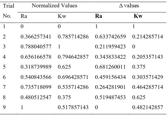
The normalized values for the surface roughness and kerf width are presented in the Table 6.

Table 6 – Normalized Values

Trial

No.

Normalized Values Δ values

Ra Kw Ra Kw

1 0 0 1 1

2 0.366257341 0.785714286 0.633742659 0.214285714

3 0.788040577 1 0.211959423 0

4 0.656166578 0.794642857 0.343833422 0.205357143

5 0.318739989 0.625 0.681260011 0.375

6 0.540843566 0.696428571 0.459156434 0.303571429

7 0.735718099 0.535714286 0.264281901 0.464285714

8 0.480512547 0.375 0.519487453 0.625

9 1 0.517857143 0 0.482142857

5.2 Grey relational coefficient and grey relational grade

After pre-processing the data, a grey relation coefficient is calculated to express the relationship between the original

and comparable sequence. The grey relational coefficient ( ) can be expressed using the formulae shown in Eqn. (6)

(6)

Here η is distinguish or identification coefficient: η ε [0,1], η = 0.5 is generally used [9]. Once the grey relational

coefficients of the responses are calculated the grey relational grade ( is obtained by calculating the average of the

coefficients. The grey relational grade is defined in the Eqn. (7) and the grey relation coefficients and the grey

relational grades are tabulated in Table 7.

Table 7 - Grey relational coefficient and Grey relational grade

Trial

1 0.333333333 0.333333333 0.333333333

2 0.441017189 0.7 0.570508594

3 0.702287214 1 0.851143607

4 0.592534008 0.708860759 0.650697384

5 0.423276836 0.571428571 0.497352704

6 0.5212914 0.622222222 0.571756811

7 0.654208872 0.518518519 0.586363695

8 0.490442524 0.444444444 0.467443484

9 1 0.509090909 0.754545455

In grey relational analysis, the grey relational grade is used to show the relationship among the sequences. If the two

sequences are identical, then the value of grey relational grade is equal to 1. The grey relational grade also indicates

the degree of influence that the comparability sequence could exert over the reference sequence. Therefore, if a

particular comparability sequence is more important than the other comparability sequences to the reference

sequence, then the grey relational grade for that comparability sequence and reference sequence will be higher than

other grey relational grades. Table 7 shows the grey relational coefficients for the both responses and the grey

relational grade.

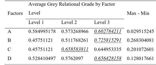
5.3 Response Table for Grey relational grade

The response table of Taguchi method is used to calculate the average grey relational grade for each factor level.

The average grey relational grade is computed by grouping the relational grades by considering the factor level for

each factors and then by taking the average of these values. The average grey relational grades (γ) for factors A and

C at level 1 and 3 respectively can be calculated as follows:

γA1 = (1/3)( 0.333333333+ 0.570508594+ 0.851143607) = 0.584995178

γC3 = (1/3)( 0.851143607+ 0.497352704+ 0.586363695) = 0.644953

Similarly calculations were performed for each factor level and response table was generated as shown in Table 8

Table 8 – Response Table

Factors

Average Grey Relational Grade by Factor

Level Max - Min

Level 1 Level 2 Level 3

A 0.584995178 0.573268966 0.602784211 0.029515245

B 0.45751121 0.511768261 0.725815291 0.268304081

C 0.45751121 0.658583811 0.644953335 0.201072601

The grey relational grades represent the correlation between the reference and the comparability sequences. The

larger the grey relational grade means the comparability sequence exhibits a stronger correlation with the reference

sequence. In Table 8, A3, B3, C2 and D3 show the largest value of grey relational grade for factors A, B, C and D

respectively. Therefore A3B3C2D3 is the optimal parameter condition for the laser cutting process, i.e. laser power is

3.5kW, cutting speed is 3.5m/min, assist gas pressure is 10 bar and standoff distance is 1mm.

When the last column of the response table shown in Table 6 is studied, it is very obvious that the difference

between the maximum and minimum grey values of the factor B i.e. cutting speed is bigger than the other three

factors, which clearly implies that the cutting speed has a stronger impact on the multi performance characteristics

than other factors.

VI. RESULTS

In the earlier steps the optimization process using GRA is done and the optimal values of the input parameters are

arrived. To make a better and quick understanding of the results, the experimentation data are presented in a

graphical way with the aid of surface graphs.

These surface graphs show the combination effect of two control factors on each response at a time. The surface

graphs clearly exhibit the change in the surface roughness or kerf width for every decrease or increase in each level

of the input parameters. The Figure 4 to Figure 7 shows the effect of the various input parameters chosen on the

output responses.

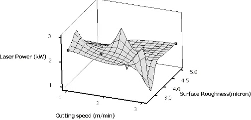
Fig. 4 – Surface graph for surface roughness Vs Laser power & cutting speed

The above figure shows clearly the effect of laser power and cutting speed on the surface roughness of the laser cut.

As the cutting speed is lesser the surface roughness is also lesser. The surface roughness dips and then rises only

slightly as there is an increase in the cutting speed. Hence the cutting speed and laser power can be maintained at

Fig. 5 – Surface graph for surface roughness Vs gas pressure & standoff distance

The inferences from the above figure are middle value of gas pressure and high value of standoff distance gives the

least surface roughness.

It is very evident from the Figure 6 that the maximum cutting speed and minimum laser power gives the optimal

kerf width.

Fig. 6 – Surface graph for kerf width Vs Laser power & cutting speed

6.1 Validation

The confirmation experiment is performed in order to prove the proposed study by using the optimal parameters

obtained using grey relational analysis technique. As shown in Table 9 the obtained response out of the optimal

parameter cutting shows a reduction in surface of around 20.64%, which is a remarkable improvement in quality.

Regarding kerf width the kerf width has improved i.e. reduced to the extent of 33% as of the average kerf width

attained in the earlier experiments.

Table 9 – Responses before and after optimization

Description γ value

Average grey relational grade before

optimization 0.581519

Grey relational grade after optimization 0.732845

VII. CONCLUSION

This paper discussed the experimental investigation on laser cutting of thick non ferrous metal sheet i.e. aluminium

alloy BS 1100 2mm thick sheet using CO2 laser. The effect of the control factors laser power, cutting speed, assist

gas pressure and standoff distance on the cut quality characteristics surface roughness and kerf width were analyzed.

The optimal parameters to obtain a better cut were obtained by optimizing the entire process using grey relational

analysis technique. The obtained results have shown considerable improvement in the quality characteristics.

This analysis can be further taken up for a detailed study on several other factors such as nozzle diameter, assist gas

etc.

REFERENCES

[1]. Pandey AK and Dubey AK, Multiple quality optimization in laser cutting of difficult-to-laser-cut material

using grey–fuzzy methodology, The International Journal of Advanced Manufacturing Technology, 65(1-4),

2013, 421-31.

[2]. A. Stournaras, P. Stavropoulos, K. Salonitis and G. Chryssolouris, An investigation of quality in CO2laser

cutting of aluminum, CIRP Journal of Manufacturing Science and Technology, 2, 2009, 61–69.

[3]. A. Riveiro, F. Quintero, F. Lusqui˜ nos, R. Comesa˜ na and J. Pou, Effects of processing parameters on laser

cutting of aluminium–copper alloys using off-axial supersonic nozzles, Applied Surface Science, 257, 2011,

5393–5397.

[4]. Amit Sharma & Vinod Yadava, Modelling and optimization of cut quality during pulsed Nd:YAG laser

cutting of thin Al-alloy sheet for curved profile, Optics and Lasers in Engineering, 51, 2013, 77–88.

[5]. Amit Sharma and Vinod Yadava, Modelling and optimization of cut quality during pulsed Nd:YAG laser

cutting of thin Al-alloy sheet for straight profile, Optics & Laser Technology, 44, 2012, 159–168.

[6]. K.Huehnlein, K. Tschirpke and R. Hellman, Optimization of laser cutting processes using design of

experiments, Physics Procedia, 5, 2010, 243–252.

[7]. Sumanta Panda, Debadutta Mishraand Bibhuti B. Biswal, Determination of Optimum Parameters With

Multi-Performance Characteristics in Laser Drilling—A Grey Relational Analysis Approach, Int J Adv Manuf

Technol, 54, 2011, 957–967

[8]. Radovanović M, Comparative modeling of CO2 laser cutting using multiple regression analysis and artificial

neural network, International Journal of Physical Sciences, 7(16), 2012, 2422-30.

[9]. Petrianu Cristian, Inţă Marinela, Manolea Daniel and Muntean Achim, Experimental Analysis and

Optimization of CO2 Laser Cutting Process for Stainless Steel Using Design of Experiments (DOE), Annals of

[10].Arun Kumar Pandey and Avanish Kumar Dubey, Simultaneous optimization of multiple quality characteristics

in laser cutting of titanium alloy sheet, Optics & Laser Technology, 44, 2012, 1858–1865.

[11].Lo KH, A comparative study on Nd: YAG laser cutting of steel and stainless steel using continuous, square,

and sine waveforms, Journal of materials engineering and performance, 21(6), 2012, 907-14.

[12].H.A. Eltawahni, M. Hagino, K.Y. Benyounis, T. Inoue and A.G. Olabi, Effect of CO2laser cutting process

parameters on edge quality and operating cost of AISI316L, Optics & Laser Technology, 44, 2012, 1068–

1082.

[13].A. Riveiro, F. Quintero, F. Lusqui˜ nos, R. Comesa˜ na and J. Pou, Parametric investigation of CO2 laser

cutting of 2024-T3 alloy, Journal of Materials Processing Technology, 210, 2010, 1138–1152.

[14].Anoop N. Samant and Narendra B. Dahotre, Computational predictions in single-dimensional laser

machining of alumina, International Journal of Machine Tools & Manufacture, 48, 2008, 1345–1353.

[15].