Recent progress in applying lattice QCD to kaon physics

Recent progress in applying lattice QCD to kaon physics

XuFeng1,2,3,⋆

1_{School of Physics and State Key Laboratory of Nuclear Physics and Technology, Peking University, Beijing} 100871, China

2_{Collaborative Innovation Center of Quantum Matter, Beijing 100871, China} 3_{Center for High Energy Physics, Peking University, Beijing 100871, China}

Abstract. Standard lattice calculations in kaon physics are based on the evaluation of matrix elements of local operators between two single-hadron states or a single-hadron state and the vacuum. Recent progress in lattice QCD has gone beyond these standard observables. I will review the status and prospects of lattice kaon physics with an empha-sis on non-leptonicK→ππdecay and long-distance processes includingK0_-K0_mixing and rare kaon decays.

1 Introduction

Since the discovery of kaons, the kaon physics plays a key role in the building of the Standard Model. The main mission for lattice QCD in kaon physics is to evaluate the low-energy hadronic effects to test the Standard Model parameters or to constrain on new physics. Lattice QCD has been successful for the calculations of the observables such as the pion and kaon decay constantsfK±_/π±, theK→πν semileptonic form factorf+(0)and the neutral kaon mixing parameterBK. We refer these observables as “standard”. Their relevant hadronic matrix elements have only one local operator insertion. The initial and final states involve at most one stable hadron. Besides, the spatial momenta carried by initial/final-state particles are much smaller than the ultraviolet lattice cutoff1_/a, witha the lattice spacing. These standard observables can be computed with high statistical precision and controlled systematic errors using lattice QCD simulations.

Many interesting observables in kaon physics, however, are not “standard”. One example is the calculation ofK→ππdecay where the final state involves multiple hadrons. Another example is the evaluation of the long-distance contributions to flavor changing processes such as the calculation of the real and imaginary parts ofK0_-K0_{mixing amplitudes, which are related to theKL-KS mass difference} ∆MKand the indirect CP violating parameter. Rare kaon decays includingK→πν¯νandK→π+− also belong to this category. As these transitions proceed via the second-order weak interaction, the calculations would involve the construction of 4-point correlation function and the treatment of non-local matrix elements with two effective operator insertions. To tackle such quantities, one needs to develop new techniques.

In this report, I will first summarize the lattice QCD calculation of standard observables. They include fK±_/π±, f₊(0), and inclusiveτ→sdecay. All these quantities are related to the determination

of the Cabibbo–Kobayashi–Maskawa (CKM) matrix element∣Vus∣. I will also discuss the current status for the computation ofBK, based on both Standard Model and beyond. In the second part of this report, I will review the lattice calculations of non-standard observables such asK→ ππdecay, K0_-K0_{mixing and rare kaon decays, presenting both recently-updated lattice results and the} newly-developed lattice methodology.

2 Lattice QCD calculation of standard observables

2.1 f+(0), fK±/fπ±and resulting∣Vus∣

According to the average from Flavor Lattice Averaging Group (FLAG), updated in Nov. 2016, lattice QCD calculations ofK3form factor f+(0)and the ratio of decay constants fK±/fπ±have reached to the precision of 0.28% and 0.25% [1]

f+(0) =0.9706(27), f_fπK±

± =1.1933(29). (1)

Meanwhile, the precision experimental measurements ofK3 and leptonic decays yield the product

∣Vus∣f+(0)[2] and the ratio∣Vus/Vud∣fK±/fπ±[2,3]

∣Vus∣f+(0) =0.2165(4), ∣Vus Vud∣

fK±

fπ± =0.2760(4). (2)

Lattice inputs off+(0)and fK±/fπ±together with the experimental data give a precise determination of the CKM matrix elements

∣Vus∣ =0.2231(7), ∣Vus

Vud∣ =0.2313(7). (3) In the Standard Model, the CKM matrix is unitary. Most stringent test of CKM unitarity is given by the first row condition

∣Vu∣2≡ ∣Vud∣2+ ∣Vus∣2+ ∣Vub∣2=1. (4) Using the results of∣Vus∣and∣Vud∣ given in Eq. (3), one finds that∣Vu∣2 = 0.9798(82), which has a 2.5σdeviation from CKM unitarity. Currently the most precise determination of∣Vud∣ =0.97420(21) is from superallowed nuclearβdecay [4,5]. Using∣Vus∣from K3 decay and∣Vud∣from nuclear β decay sharpens the unitarity test with a much smaller uncertainty. However, the deviation is still around 2.4σ, as shown in the second line of Eq. (5). If using∣Vus/Vud∣from leptonic decays and∣Vud∣ from nuclearβdecay, then the result confirms the CKM unitarity; see the third line of Eq. (5). The above tests of CKM unitarity are put together here for a comparison

∣Vu∣2=⎧⎪⎪⎪⎪⎨⎪⎪⎪

⎪⎩

0.9798(82), K3+leptonic decays, 0.9988(5), K3+nuclearβdecay, 0.9998(5), leptonic+nuclearβdecay.

(5)

of the Cabibbo–Kobayashi–Maskawa (CKM) matrix element∣Vus∣. I will also discuss the current status for the computation ofBK, based on both Standard Model and beyond. In the second part of this report, I will review the lattice calculations of non-standard observables such asK →ππdecay, K0_-K0_{mixing and rare kaon decays, presenting both recently-updated lattice results and the} newly-developed lattice methodology.

2 Lattice QCD calculation of standard observables

2.1 f+(0), fK±/fπ± and resulting∣Vus∣

According to the average from Flavor Lattice Averaging Group (FLAG), updated in Nov. 2016, lattice QCD calculations ofK3 form factor f+(0)and the ratio of decay constants fK±/fπ±have reached to the precision of 0.28% and 0.25% [1]

f+(0) =0.9706(27), f_fπK±

± =1.1933(29). (1)

Meanwhile, the precision experimental measurements ofK3 and leptonic decays yield the product

∣Vus∣f+(0)[2] and the ratio∣Vus/Vud∣fK±/fπ±[2,3]

∣Vus∣f+(0) =0.2165(4), ∣Vus Vud∣

fK±

fπ± =0.2760(4). (2)

Lattice inputs of f+(0)and fK±/fπ±together with the experimental data give a precise determination of the CKM matrix elements

∣Vus∣ =0.2231(7), ∣Vus

Vud∣ =0.2313(7). (3) In the Standard Model, the CKM matrix is unitary. Most stringent test of CKM unitarity is given by the first row condition

∣Vu∣2≡ ∣Vud∣2+ ∣Vus∣2+ ∣Vub∣2=1. (4) Using the results of∣Vus∣and∣Vud∣given in Eq. (3), one finds that∣Vu∣2 = 0.9798(82), which has a 2.5σdeviation from CKM unitarity. Currently the most precise determination of∣Vud∣ =0.97420(21) is from superallowed nuclearβdecay [4,5]. Using∣Vus∣ fromK3 decay and∣Vud∣ from nuclearβ decay sharpens the unitarity test with a much smaller uncertainty. However, the deviation is still around 2.4σ, as shown in the second line of Eq. (5). If using∣Vus/Vud∣from leptonic decays and∣Vud∣ from nuclearβdecay, then the result confirms the CKM unitarity; see the third line of Eq. (5). The above tests of CKM unitarity are put together here for a comparison

∣Vu∣2=⎧⎪⎪⎪⎪⎨⎪⎪⎪

⎪⎩

0.9798(82), K3+leptonic decays, 0.9988(5), K3+nuclearβdecay, 0.9998(5), leptonic+nuclearβdecay.

(5)

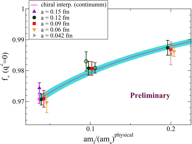
To clarify the 2.xσdeviation in the unitarity test, it is important to reduce the uncertainty from the lattice QCD determination off+(0). One of the recent updates forf+(0)is from Fermilab Lattice-MILC collaboration. HISQ fermions on 2+1+1 flavor Lattice-MILC configurations are used in the calculation and preliminary results are shown in Fig. 1. Compared to their report last year [6], more lattice ensembles are used in the analysis. Employing 4 ensembles at the physical pion mass and 2 ultra-fine

lattice spacings (0.06 and 0.042 fm) allows them to reduce the statistical error to 0.14%. At 0.12 fm andml/ms=0.1, they use three different volumes. Three volumes together with one-loop chiral perturbation theory (ChPT) [7] allow for a good estimate of the finite-volume effects. After chiral and continuum extrapolation, the total uncertainty is expected to be reduced to 0.2%, which is close to the current experimental uncertainty [2].

0.1

0.2

am

/(am

)

0.97

0.98

0.99

1

f

(q

2

=0)

chiral interp. (continumm) a = 0.15 fm

a = 0.12 fm a = 0.09 fm a = 0.06 fm a = 0.042 fm

Preliminary

Figure 1.Form factor f+(0)vs. light-quark mass from Fermilab Lattice-MILC collaboration. The calculation is performed at 5 lattice spacings 0.15, 0.12, 0.09, 0.06 and 0.042 fm, including 4 ensembles with physical pion mass. Open green symbols correspond to different volumes for a=0.12 fm andml =0.1ms. The solid magenta

line is the (preliminary) interpolation in the light-quark mass, keeping the strange-quark massms equal to its physical value, and turning offall discretization effects. The magenta diamond is the corresponding interpolation

at the physical point. Data at the same light-quark mass but different lattice spacing are off-set horizontally.

Another lattice calculation is recently reported by JLQCD collaboration [8,9]. In their calculation, the chiral symmetry is exactly preserved by using the overlap quark action, which enables a direct comparison of the lattice data with ChPT and hence a determination of relevant low energy constants within NNLO ChPT. A reasonable agreement between lattice results for the sloped f+(q2)/dq2 (at q2_{=0) and experiment is observed, although the error is still large due to the high cost of the usage} of overlap fermion.

2.2 τinclusive decay and∣Vus∣

To explore the discrepancy, the main quantity of interest is the ratio of the decay rates

R₌ Γ(τ→s-hadronsντ) Γ(τ→eνeν¯ τ)

, (6)

whereτ → s-hadronsντ indicates that in the decay the final-state hadrons contain net strange-ness. According to the optical theorem, the imaginary part of the hadronic vacuum polarization (HVP) functions can be related to theR-value through [12]

dR ds =

12π∣Vus∣2SEW m2

τ (

1−_ms₂

τ) 2

[(1+2 s m2

τ)

ImΠ(1)(s) +ImΠ(0)(s)], (7)

wheresis the invariant mass square of the final-state hadrons. SEW is a known short-distance elec-troweak correction [13]. Π(J)(s)are the HVP functions with the superscript (J)corresponding to angular momentaJ₌0,1.

Once ImΠ(J)(s)is known, Eq. (7) can be used to determine∣Vus∣. Since ImΠ(J)(s)is generically non-perturbative at smalls, the conventional approach to determine ImΠ(J)(s)is to use the dispersion relation [12]

∫_4ms02

π

ds W(s)ImΠ(s) =₂i _∮

∣s∣=s0

ds W(s)Π(s), (8)

where ImΠ(s)on the left-hand side can be related todR/dsand∣Vus∣, while the integral on the right-hand side can be determined using QCD perturbation theory (pQCD) and operator product expansion (OPE). The parameters0should be sufficiently large for a good convergence of pQCD and the validity of the OPE.W(s)is a weight function. If there is no pole inside the contour, then the integral along the branch cut is equal to the integral on the circle and then∣Vus∣ can be determined. A difficulty here is that the estimate of high-dimensional OPE terms relies on some assumptions and thus contains potentially large systematic effects. Using the conventional approach described above, it results in the low value of∣Vus∣shown in the left panel of Fig.2[14].

An improvement is proposed by Ref. [15] to use different s₀ and weight functions W(s) and then study the dependence on s0 andW(s). Through fit, not only∣Vus∣, but also the OPE effective condensates are fit to experimental measurements (and also lattice QCD data). With this improvement, the 3.2σdeviation is reduced to 1-2 σlevel depending on using BaBar or 2014 HFAG result for Br_[τ−→K−π0ντ]

∣Vus∣ =⎧⎪⎪⎨⎪⎪

⎩

0.2229(22) using BaBarτ−→K−π0ντ, 3.2σ→1.2σ, 0.2204(23) using HFAGτ−→K−π0ντ, 3.2σ→2.2σ.

(9)

These results are plotted on the right-panel of Fig.2, denoted as “τFB FESR, HLMZ17”.

Another new approach proposed by H. Ohki et. al. [16] is to let s0 → ∞ and use the weight function containing the pole structures

W(s) =∏N

k=1 1 s₊Q2

k

, (10)

where theNdifferent polesQ2

kare spanned by a spacing∆=0.2/(N−1)GeV2, with a center point calledC. OnceW(s)is given, the contour of the integral is equal to the residues of the poles, which can be determined using lattice HVPs. Thus the value of∣Vus∣can be determined accordingly. The strategy to chooseQ2

To explore the discrepancy, the main quantity of interest is the ratio of the decay rates

R₌ Γ(τ→s-hadronsντ) Γ(τ→eνeν¯ τ)

, (6)

whereτ → s-hadronsντindicates that in the decay the final-state hadrons contain net strange-ness. According to the optical theorem, the imaginary part of the hadronic vacuum polarization (HVP) functions can be related to theR-value through [12]

dR ds =

12π∣Vus∣2SEW m2

τ (

1−_ms₂

τ) 2

[(1+2 s m2

τ)

ImΠ(1)(s) +ImΠ(0)(s)], (7)

wheresis the invariant mass square of the final-state hadrons. SEW is a known short-distance elec-troweak correction [13]. Π(J)(s)are the HVP functions with the superscript (J)corresponding to angular momentaJ₌0,1.

Once ImΠ(J)(s)is known, Eq. (7) can be used to determine∣Vus∣. Since ImΠ(J)(s)is generically non-perturbative at smalls, the conventional approach to determine ImΠ(J)(s)is to use the dispersion relation [12]

∫_4ms02

π

ds W(s)ImΠ(s) = i 2∮∣s∣=s0

ds W(s)Π(s), (8)

where ImΠ(s)on the left-hand side can be related todR/dsand∣Vus∣, while the integral on the right-hand side can be determined using QCD perturbation theory (pQCD) and operator product expansion (OPE). The parameters0should be sufficiently large for a good convergence of pQCD and the validity of the OPE.W(s)is a weight function. If there is no pole inside the contour, then the integral along the branch cut is equal to the integral on the circle and then∣Vus∣can be determined. A difficulty here is that the estimate of high-dimensional OPE terms relies on some assumptions and thus contains potentially large systematic effects. Using the conventional approach described above, it results in the low value of∣Vus∣shown in the left panel of Fig.2[14].

An improvement is proposed by Ref. [15] to use different s₀ and weight functions W(s) and then study the dependence on s0 andW(s). Through fit, not only ∣Vus∣, but also the OPE effective condensates are fit to experimental measurements (and also lattice QCD data). With this improvement, the 3.2σ deviation is reduced to 1-2σlevel depending on using BaBar or 2014 HFAG result for Br_[τ−→K−π0ντ]

∣Vus∣ =⎧⎪⎪⎨⎪⎪

⎩

0.2229(22) using BaBarτ−→K−π0ντ, 3.2σ→1.2σ, 0.2204(23) using HFAGτ−→K−π0ντ, 3.2σ→2.2σ.

(9)

These results are plotted on the right-panel of Fig.2, denoted as “τFB FESR, HLMZ17”.

Another new approach proposed by H. Ohki et. al. [16] is to let s0 → ∞ and use the weight function containing the pole structures

W(s) =∏N

k=1 1 s₊Q2

k

, (10)

where theNdifferent polesQ2

kare spanned by a spacing∆=0.2/(N−1)GeV2, with a center point calledC. OnceW(s)is given, the contour of the integral is equal to the residues of the poles, which can be determined using lattice HVPs. Thus the value of∣Vus∣can be determined accordingly. The strategy to chooseQ2

k is that it should not be too large to suppress the contribution from pQCD and

|

us

|V

0.22 0.225

, PDG 2016

l3

K

0.0010 ± 0.2237

, PDG 2016

l2

K

0.0007 ± 0.2254

CKM unitarity, PDG 2016 0.0009

±

0.2258

s incl., HFLAV Spring 2017 →

τ

0.0021 ± 0.2186

, HFLAV Spring 2017 ν π → τ / ν K → τ 0.0018 ± 0.2236

average, HFLAV Spring 2017 τ

0.0015 ± 0.2216

HFLAV

Spring 2017 0.215 0.22 0.225|V_us|0.23 0.235 0.24

K_l3, PDG 2016

Γ[K_µ2]

3-family unitarity, HT14 |V_ud|

τ FB FESR, HFAG17

τ FB FESR, HLMZ17

τ, lattice [N=3, C=0.3 GeV2]

τ, lattice [N=4, C=0.7 GeV2]

τ, lattice [N=5, C=0.9 GeV2_]

(conventional implementation)

(new implementation, lower : HFAG16 input)

this work (preliminary)

Figure 2. Left: HFLAV summary of∣Vus∣. For the τ → sinclusive decay, there is a 3.2σdeviation from CKM unitarity. Right: New implementations forτ→ sinclusive decay. The read circle data points, denoted as “τFB FESR, HLMZ17”, show the improvement by fitting the OPE effective condensates to the experimental

measurements and lattice QCD data [15]. The green square data points show the improvement usingW(s)in Eq. (10) and using lattice HVPs for the residues of the integral [16]. Both improvements shed light on the resolution of the puzzle from theτ→sinclusive decay.

OPE at s > m2

τ. It should not be too small to avoid large statistical error from lattice HVPs. The realistic calculation is performed usingNf=2+1 Möbius domain wall fermions at near-physical pion mass with the lattice spacingsa−1 =1.73 and 2.36 GeV and the lattice volume V = (5 fm)3_{. The} corresponding results are summarized in the right panel of Fig.2, denoted by the green square data points (The filled-square points are generated usingτ → Kντdata for the K pole, while the open-square ones use theKµ2 data as input). Using different N andC, the lattice calculation shows the consistent results. Besides, all the data points are systematically larger than the conventional value of

∣Vus∣. AtN=4 andC=0.7 GeV2,∣Vus∣is obtained as

∣Vus∣ =⎧⎪⎪⎨⎪⎪

⎩

0.2228(21), usingτ→Kντinput for theKpole

0.2245(16), usingKµ2input for theKpole. (11)

Both improvements proposed by Refs. [15] and [16] shed light on the resolution of the puzzle from theτ→sinclusive decay.

2.3 Neutral-kaon mixing parameterBK based on Standard Model and beyond

The parameterBKis related to the CP violating part ofK0-K0mixing and thus short-distance domi-nated. Using OPE, the effective HamiltonianH∆S=2

eff can be written as a product of the Wilson

coeffi-cientC(µ)and the∆S =2 local operatorQ∆S=2(_µ)

H∆S=2

eff =

G2 FM2W 16π2 C(µ)Q

∆S=2_{(µ), (12)}

withGFthe Fermi constant andMWtheW-boson mass. It is a convention to use the parameteras a measure of indirect CP violation,

= A(KL→ (ππ)I=0)

with the initial state given byKL/S particle and the final state having total isospin zero. The contribu-tion fromH∆S=2

eff serves as a dominant contribution to

=exp(iφ)sin(φ) [

Im[MSD ¯00] ∆MK +

Im[MLD ¯00] ∆MK +

Im[A0] Re[A0]], M

SD

¯00 = ⟨K0∣He∆ffS=2∣K0⟩. (14)

Here the angleφ ≡ arctan(−2∆MK/∆ΓK) ≈43.52(5)○[11], with∆MK = MKL−MKS and∆ΓK = ΓK_L−ΓK_S. MLD_¯00 indicates the long-distance contribution toandA0is theK0→ (ππ)I=0amplitude. BothMLD

¯00 andA0only make few-percent contributions to. The progress in lattice QCD calculation of these two quantities will be discussed later. Here we only focus on theMSD

¯00. Within Standard Model, there is only one∆S =2 operator withV−Astructure

Q∆S=2= [_{sα¯ γ}

µ(1−γ5)dα] [sβ¯ γµ(1−γ5)dβ], (15)

where the subscriptsαandβdenote the color indices. For beyond-Standard-Model theories, 4 other operators are possible

Q∆S=2

2 = [sα¯ (1−γ5)dα] [sβ¯ (1−γ5)dβ], Q3∆S=2= [sα¯ (1−γ5)dβ] [sβ¯ (1−γ5)dα], Q∆S=2

4 = [sα¯ (1−γ5)dα] [sβ¯ (1+γ5)dβ], Q5∆S=2= [sα¯ (1−γ5)dβ] [sβ¯ (1+γ5)dα]. (16) The neutral-kaon mixing parameterBKandBiin the MS scheme are defined as

BK(µ) = ⟨K

0_∣Q∆S=2(_µ)∣_K0⟩

8 3fK2MK2

,

Bi(µ) = ⟨K 0_∣Q∆S=2

i (µ)∣K0⟩ Ni⟨K0∣s¯γ5d∣0⟩⟨0∣s¯γ5d∣K0⟩

, {N2,⋯,N5} = {−5/3,1/3,2,2/3}, (17)

whereµis the renormalization scale, fK the kaon decay constant and MK the kaon mass. Given the anomalous dimensionγ(g), the renormalization group independentBparameter ˆBK is related to BK(µ)by the formula

ˆ

BK= (g¯(µ) 2

4π ) −γ0/(2β0)

exp_{∫ g¯(µ) 0 dg(

γ(g) β(g) +

γ0

β0g)}BK(µ). (18)

For the Standard Model ˆBK, the lattice calculation has reached a precision of 1.3% for 2+1 flavor calculation [1]

ˆ

BK=0.763(10). (19)

For beyond-Standard-ModelBi(µ)at the MS scaleµ=3 GeV, the uncertainties of 2+1 flavor lattice results are about 2-5% [1]

B2=0.502(14), B3=0.766(32), B4=0.926(19), B5=0.720(38). (20)

The results forBi(µ)from various groups are summarized by FLAG [1] on the top panel of Fig.3. There are clear discrepancies inB4andB5from different groups. To resolve these discrepancies, RBC-UKQCD collaboration undertakes a study using both RI-MOM and RI-SMOM renormalization [17–

with the initial state given byKL/S particle and the final state having total isospin zero. The

contribu-tion fromH∆S=2

eff serves as a dominant contribution to

=exp(iφ)sin(φ) [

Im[MSD ¯00] ∆MK +

Im[MLD ¯00] ∆MK +

Im[A0]

Re[A0]], M SD

¯00 = ⟨K0∣H∆effS=2∣K0⟩. (14) Here the angleφ ≡ arctan(−2∆MK/∆ΓK) ≈ 43.52(5)○[11], with∆MK = MKL −MKS and∆ΓK =

ΓKL−ΓKS. MLD¯00 indicates the long-distance contribution toandA0is theK0→ (ππ)I=0amplitude.

BothMLD

¯00 andA0only make few-percent contributions to. The progress in lattice QCD calculation

of these two quantities will be discussed later. Here we only focus on theMSD ¯00.

Within Standard Model, there is only one∆S =2 operator withV−Astructure

Q∆S=2= [_s¯

αγµ(1−γ5)dα] [s¯βγµ(1−γ5)dβ], (15)

where the subscriptsαandβdenote the color indices. For beyond-Standard-Model theories, 4 other operators are possible

Q∆S=2

2 = [s¯α(1−γ5)dα] [s¯β(1−γ5)dβ], Q₃∆S=2= [s¯α(1−γ5)dβ] [s¯β(1−γ5)dα],

Q∆S=2

4 = [s¯α(1−γ5)dα] [s¯β(1+γ5)dβ], Q5∆S=2= [s¯α(1−γ5)dβ] [s¯β(1+γ5)dα]. (16) The neutral-kaon mixing parameterBKandBiin the MS scheme are defined as

BK(µ) = ⟨K

0_∣Q∆S=2(_µ)∣_K0⟩

8 3fK2M2K

,

Bi(µ) = ⟨K 0_∣Q∆S=2

i (µ)∣K0⟩ Ni⟨K0∣s¯γ5d∣0⟩⟨0∣s¯γ5d∣K0⟩

, {N2,⋯,N5} = {−5/3,1/3,2,2/3}, (17)

whereµ is the renormalization scale, fK the kaon decay constant and MK the kaon mass. Given

the anomalous dimensionγ(g), the renormalization group independentBparameter ˆBK is related to BK(µ)by the formula

ˆ

BK= (g¯(µ) 2

4π ) −γ0/(2β0)

exp_{∫ g¯(µ)

0 dg( γ(g) β(g) +

γ0

β0g)}BK(µ). (18)

For the Standard Model ˆBK, the lattice calculation has reached a precision of 1.3% for 2+1 flavor

calculation [1]

ˆ

BK=0.763(10). (19)

For beyond-Standard-ModelBi(µ)at the MS scaleµ=3 GeV, the uncertainties of 2+1 flavor lattice

results are about 2-5% [1]

B2=0.502(14), B3=0.766(32), B4=0.926(19), B5=0.720(38). (20)

The results forBi(µ)from various groups are summarized by FLAG [1] on the top panel of Fig.3.

There are clear discrepancies inB4andB5from different groups. To resolve these discrepancies,

RBC-UKQCD collaboration undertakes a study using both RI-MOM and RI-SMOM renormalization [17–

19]. The calculation is performed usingNf =2+1 flavor domain wall fermion at Mπ ≈ 300 MeV and two lattice spacingsa=0.08 and 0.11 fm. The corresponding results are shown by the three data

points below the legend of “RBC-UKQCD ’16” on the bottom panel of Fig.3, where the four red data

1.0

0.8

0.6

0.4

B₄

Figure 3. Top: FLAG summary ofBi(µ)atµ =3 GeV [1]. There are clear discrepancies inB4and B5from different groups. Bottom: Comparison forB4 using RI-MOM and RI-SMOM non-perturbative renormalization and 1-loop perturbative renormalization. The four red data points use RI-MOM scheme while the two green ones use RI-SMOM scheme and the orange one uses 1-loop lattice perturbation theory. All RI-MOM results are compatible among different groups. However, they are systematically smaller than the RI-SMOM and 1-loop

points use RI-MOM scheme while the two green ones use RI-SMOM scheme and the orange one uses 1-loop lattice perturbation theory. Including the new RBC-UKQCD updates, all RI-MOM results are compatible among different groups. However, these results are systematically smaller than that from the RI-SMOM renormalization and the 1-loop lattice perturbation theory. Particularly for RI-SMOM calculation, both_(/q,_/q)and(γ, γ)-schemes are used and consistent results (shown by the two green data points) are obtained after conversion to MS scheme. ForB5, the situation is very similar.

According to the study by Ref. [20], RI-SMOM renormalization is expected to have smaller in-frared contamination than RI-MOM due to the usage of the non-exceptional momenta. The studies by [17–19] confirm such expectation and suggest that forB4andB5RI-SMOM renormalization should be used to fully control the infrared contamination. In Ref. [21] an update is reported on the RBC-UKQCD measurement ofBi(µ), simulated using Nf = 2+1 domain wall fermions at the physical quark masses.

3 Go beyond standard observables

3.1 K→ππdecay and direct CP violation

CP violation was first observed in neutral kaon decays. Under CP transform, theK0_{state is related to} K0_{state through}

CP∣K0⟩ = −∣K0_{⟩. (21)}

The CP eigenstate can be defined as the combination ofK0_andK0

K0

±= √1₂(K0∓K0), (22)

withK0

+/−the CP-even/odd state. The physical states observed in the experiment are the weak eigen-states KS and KL. KS decays into two pions and KL decays into three pions. By neglecting CP violation,KS is equal to CP-even state andKLequal to CP-odd state. In 1964, BNL discovered that KLis able to decay into two pions, indicating the violation of CP symmetry. This discovery leads to the Nobel prize in 1980.

SinceKLandKS are not CP eigenstates, one can write them as a mixture of the CP eigenstates

∣KL/S⟩ = √ 1 1+¯2(∣K

0

∓⟩ +¯∣K0±⟩). (23)

The parameter ¯is a measure of the strength of mixing. ForKL→ππdecay, there are two contributions to the CP violation. The first part appears as the CP-even component ofKL decays into two pions. This is called indirect CP violation and described by a parameteror in many cases written asK. receives its dominant contribution from ¯and a small contribution fromA0due to its definition given in Eq. (13)

=¯+iIm[A0]

Re[A0]. (24)

The second contribution is from the CP-odd component ofKL, which decays into two pions directly. This is called direct CP violation and denoted as′.

The experiments measure the decay amplitudes ofKL→ππandKS →ππand use the ratio

η+−≡ A(KL→π +_π−₎ A(KS →π+π−) ≡+

′_{, η}

00≡ A(KL→π 0_π0₎

A(KS →π0π0) ≡−2

points use RI-MOM scheme while the two green ones use RI-SMOM scheme and the orange one uses 1-loop lattice perturbation theory. Including the new RBC-UKQCD updates, all RI-MOM results are compatible among different groups. However, these results are systematically smaller than that from

the RI-SMOM renormalization and the 1-loop lattice perturbation theory. Particularly for RI-SMOM calculation, both_(/q,_/q)and(γ, γ)-schemes are used and consistent results (shown by the two green data points) are obtained after conversion to MS scheme. ForB5, the situation is very similar.

According to the study by Ref. [20], RI-SMOM renormalization is expected to have smaller in-frared contamination than RI-MOM due to the usage of the non-exceptional momenta. The studies by [17–19] confirm such expectation and suggest that forB4andB5RI-SMOM renormalization should

be used to fully control the infrared contamination. In Ref. [21] an update is reported on the RBC-UKQCD measurement ofBi(µ), simulated using Nf = 2+1 domain wall fermions at the physical

quark masses.

3 Go beyond standard observables

3.1 K→ππdecay and direct CP violation

CP violation was first observed in neutral kaon decays. Under CP transform, theK0_{state is related to} K0_{state through}

CP∣K0⟩ = −∣K0_{⟩. (21)}

The CP eigenstate can be defined as the combination ofK0_andK0

K0

±= √1₂(K0∓K0), (22)

withK0

+/−the CP-even/odd state. The physical states observed in the experiment are the weak

eigen-states KS and KL. KS decays into two pions and KL decays into three pions. By neglecting CP

violation,KS is equal to CP-even state andKLequal to CP-odd state. In 1964, BNL discovered that KLis able to decay into two pions, indicating the violation of CP symmetry. This discovery leads to

the Nobel prize in 1980.

SinceKLandKS are not CP eigenstates, one can write them as a mixture of the CP eigenstates

∣KL/S⟩ = √ 1

1+¯2(∣K

0

∓⟩ +¯∣K±0⟩). (23)

The parameter ¯is a measure of the strength of mixing. ForKL→ππdecay, there are two contributions

to the CP violation. The first part appears as the CP-even component ofKLdecays into two pions.

This is called indirect CP violation and described by a parameteror in many cases written asK.

receives its dominant contribution from ¯and a small contribution fromA0due to its definition given

in Eq. (13)

=¯+iIm[A0]

Re[A0]. (24)

The second contribution is from the CP-odd component ofKL, which decays into two pions directly.

This is called direct CP violation and denoted as′.

The experiments measure the decay amplitudes ofKL→ππandKS →ππand use the ratio

η+−≡ A(KL→π +_π−₎ A(KS →π+π−) ≡+

′_{, η}

00≡ A(KL→π 0_π0₎

A(KS →π0π0) ≡−2

′ ₍₂₅₎

Current-current

Q1,Q2

QCD penguin

Q3-Q6

Electro-weak penguin

Q7-Q10

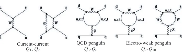
Figure 4. Examples of current-current, QCD penguin and electroweak penguin diagrams in the full theory for

K→ππdecays.

to determine the parameterand′. Using the experimental measurements of∣η₊₋∣and∣η00∣as input,

PDG quotes [11]

∣∣ ≈ 1

3(2∣η+−+ ∣η00∣) =2.228(11) ×10−3, Re[′/] ≈ 1 3(1− ∣

η00∣

∣η+−∣) =1.66(23) ×10

−3_{. (26)}

is at the order of 10−3and′is even 1000 times smaller. Due to its small size, direct CP violation′

is very sensitive to new physics.

For theoretical simplicity, it is convenient to study the decay amplitudes in the specific isospin channels,A0andA2,

A(K0_{→ (ππ)}

I) =AIeiδI, I=0,2, (27)

whereδIis the strong phase fromππscattering. If CP symmetry were protected, then both the

ampli-tudesA2andA0are real. To obtain the CP violation, one shall determine both real and imaginary part

ofA2andA0. The indirect CP violationonly has a small dependence onA0as shown by Eq. (24).

While for′, it is sensitive on both real and imaginary part ofA2andA0

′= ie i(δ2−δ0)

√

2

Re[A2]

Re_[A0] (

Im[A2]

Re_[A2] −

Im[A0]

Re_[A0]). (28)

The target for lattice QCD calculation is to determineA2andA0from first principles.

The weak Hamiltonian forK→ππdecay is given by a series of∆S =1 local four-quark

opera-tors [22]

H∆S=1 eff =

GF

√

2VudV

∗ us

10

∑

i=1[zi(µ) +τyi(µ)]Qi. (29)

Hereτ= −VtdVts∗

VudVus∗ =1.543+0.635iis the ratio of CKM matrix elements. zi(µ)andyi(µ)are known

perturbative Wilson coefficients that summarize the short-distance effects. The 10 local four-quark

operatorsQican be matched to three types of diagrams in the full theory, shown in Fig. 4with the

notations “Current-current”, “QCD penguin” and “Electro-weak penguin”, respectively. Q1,Q2are

current-current operators, which dominate the contribution to Re[A2]and Re[A0]. Q3-Q6 are QCD

penguin operators, whereQ6dominates the contribution to Im[A0].Q7-Q10are electroweak penguin

operators, which dominate the contribution to Im[A2].

The most recent updated results for the amplitude A2 are given by RBC-UKQCD

The parameters are given in Table1. After continuum extrapolation the results forA2are given by

Re_[A2] =1.50(4)stat(14)syst×10−8GeV, Im[A2] = −6.99(20)stat(84)syst×10−13GeV, (30)

where Re[A2]is consistent with the experimental measurement of Re[A2] ≈ ∣A2∣ =1.479(3) ×10−8 GeV obtained fromK+ decays. For Im[A2], it is unknown from experiments. Only lattice QCD provides the result. For theI=2ππscattering phase atEππ=MK, the lattice calculation yields

δ2= −11.6(2.5)(1.2)○ (31)

which is calculated using Lüscher’s formula [24] and consistent with the phenomenological curve from Ref. [25].

Table 1.Ensembles used in the recent lattice calculation ofA2by RBC-UKQCD collaboration [23].

Mπ(MeV) (L/a)3× (T/a) a(fm) L(fm) Nconf

139.1(2) 483_{×96 0.11 5.4 76}

139.2(3) 643_{×128 0.084 5.4 40}

In addition to the determination ofA2andδ2, another outcome from Ref. [23] is the resolution of the puzzle of the∆I=1/2 rule. According to experimental measurement, the size ofA₀is about 22.5 times larger than that ofA2. It is a more-than-half-century’s puzzle since 1955 [26] on why the am-plitudes in the different isospin channels are so much different. The Wilson coefficients only account for a factor of 2. The lattice calculation shows that Re[A2]is dominated by diagramsC1andC2in the left panel of Fig.5, whereC1is color diagonal andC2color mixed.C2is 1/Nsuppressed relative to C1withC2equal to 1/3 ofC1in leading order QCD perturbation theory. However, the lattice results in the right panel of Fig.5shows thatC2is about−0.7×C1, indicating very strong non-perturbative effects. As Re[A2]is proportional toC1+C2, the observation thatC1 andC2 have opposite signs leads to a significant cancellation between the two terms. While for Re[A0], the opposite signs lead to an enhancement as Re[A0]receives an important contribution from 2C1−C2. When considering the complete contribution to Re[A0], including the disconnected diagrams, the size of Re[A0]is more enhanced. In total, the hadronic matrix elements including the contributions fromC1,C2and other diagrams would contribute another factor of∼ 10. The cancellation betweenC1 andC2 was first observed in an earlier study [27] and further confirmed by the latest calculation ofA2[23]. So now the puzzle of∆I=1/2 rule is resolved from first principles. We have also seen a recent study of the ∆I=1/2 rule with the scaling of the number of color [28].

The more demanding calculation is theK _→ ππdecay in the isopsinI = 0 channel. The latest calculation is performed at the physical kinematicsMπ=143.1(2.0)MeV andMK=490(2.2)MeV, using a 323_{×64 lattice volume and a lattice spacinga=0.14 fm [29]. G-parity boundary condition is} used and the lattice volume is chosen such that the kaon’s mass is equal to the pion-pion’s energy in the ground state. Based on 216 configurations, the lattice results for Re[A0]and Im[A0]are reported as

The parameters are given in Table1. After continuum extrapolation the results forA2are given by

Re_[A2] =1.50(4)stat(14)syst×10−8GeV, Im[A2] = −6.99(20)stat(84)syst×10−13GeV, (30)

where Re[A2]is consistent with the experimental measurement of Re[A2] ≈ ∣A2∣ = 1.479(3) ×10−8 GeV obtained fromK+ decays. For Im[A2], it is unknown from experiments. Only lattice QCD provides the result. For theI=2ππscattering phase atEππ=MK, the lattice calculation yields

δ2= −11.6(2.5)(1.2)○ (31)

which is calculated using Lüscher’s formula [24] and consistent with the phenomenological curve from Ref. [25].

Table 1.Ensembles used in the recent lattice calculation ofA2by RBC-UKQCD collaboration [23].

Mπ(MeV) (L/a)3× (T/a) a(fm) L(fm) Nconf

139.1(2) 483_{×96 0.11 5.4 76}

139.2(3) 643_{×128 0.084 5.4 40}

In addition to the determination ofA2andδ2, another outcome from Ref. [23] is the resolution of the puzzle of the∆I=1/2 rule. According to experimental measurement, the size ofA₀is about 22.5 times larger than that ofA2. It is a more-than-half-century’s puzzle since 1955 [26] on why the am-plitudes in the different isospin channels are so much different. The Wilson coefficients only account for a factor of 2. The lattice calculation shows that Re[A2]is dominated by diagramsC1andC2in the left panel of Fig.5, whereC1is color diagonal andC2color mixed.C2is 1/Nsuppressed relative to C1withC2equal to 1/3 ofC1in leading order QCD perturbation theory. However, the lattice results in the right panel of Fig.5shows thatC2is about−0.7×C1, indicating very strong non-perturbative effects. As Re[A2]is proportional toC1+C2, the observation thatC1 andC2 have opposite signs leads to a significant cancellation between the two terms. While for Re[A0], the opposite signs lead to an enhancement as Re[A0]receives an important contribution from 2C1−C2. When considering the complete contribution to Re[A0], including the disconnected diagrams, the size of Re[A0]is more enhanced. In total, the hadronic matrix elements including the contributions fromC1,C2 and other diagrams would contribute another factor of∼ 10. The cancellation betweenC1 andC2 was first observed in an earlier study [27] and further confirmed by the latest calculation ofA2[23]. So now the puzzle of∆I=1/2 rule is resolved from first principles. We have also seen a recent study of the ∆I=1/2 rule with the scaling of the number of color [28].

The more demanding calculation is theK _→ ππdecay in the isopsinI = 0 channel. The latest calculation is performed at the physical kinematicsMπ=143.1(2.0)MeV andMK=490(2.2)MeV, using a 323_{×64 lattice volume and a lattice spacinga=0.14 fm [29]. G-parity boundary condition is} used and the lattice volume is chosen such that the kaon’s mass is equal to the pion-pion’s energy in the ground state. Based on 216 configurations, the lattice results for Re[A0]and Im[A0]are reported as

Re[A0] =4.66(1.00)stat(1.26)syst×10−7GeV, Im[A0] = −1.90(1.23)stat(1.08)syst×10−11GeV. (32) Here the real part is consistent with the experimental result: Re[A0] =3.3201(18) ×10−7GeV. The experimental value of Im[A0]does not exist, and the knowledge is only from lattice. Using Lüscher’s quantization condition [24], theI=0ππscattering phase shift is found to beδ0 =23.8(4.9)(1.2)○, which is smaller than the valueδ0 =38.0(1.3)○, obtained by combining experimental data with the

K

π

π i

j j

i

C1: color diagonal

K

π

π j

j i

i

C2: color mixed

0 1 2 3 4 5 6 7 8 9

0 5 10 15 20 25 30 35

Contraction (x10

6 )

t

C₁ -C₂ C₁+C₂

Figure 5.Left: Dominant contractions contributing to Re[A2]. Right: Cancellation ofC1andC2-contributions to Re_[A2]at the physical pion mass anda=0.084 fm.

Roy equations [30,31]. It remains a puzzle for the discrepancy and needs to be understood in the future study.

Using the lattice results for bothA0andA2, the direct CP violation′/can be determined:

Re[′/] =0.14(52)stat(46)syst×10−3. (33)

There is a 2.1σdeviation from experimental value Re[′/] =1.66(23)×10−3[32]. As the uncertain-ties of the lattice results are larger than experimental measurement, to confirm whether new physics information can be found in the deviation, more accurate lattice calculations are required.

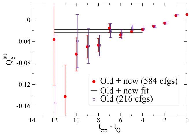
It is reported by C. Kelly [33] that the statistics of the previous RBC-UKQCD calculation has been increased to 584 configurations. In the lattice calculation, the largest contribution to Im[A0]comes fromQ6 operator. Fig.6shows the fit to obtain the matrix element⟨ππ∣Q6∣K⟩. When the statistics increases from 216 to 584 configurations, uncertainty decreases as expected while the central values remain consistent. The aim of the RBC-UKQCDK→ππprogram is to reduce the dominant statistical error for Re[′/]in Eq. (33) by a factor of 2 within the next year.

Besides for the effort to increase the statistics, there are also efforts for improvements of various systematic effects. For example, theσfield starts to be added into the calculation to account for the σ → ππeffects in theI = 0 ππscattering channel. In Ref. [34] N. H. Christ reports on including electromagnetism inK_→ππdecay. The∆I=1/2 rule may make the effects of electromagnetism on A2∼20 times larger than a naiveO(αe)estimate due to the mixing withA0. Such effects will become important if the target of the future calculations is to determine′/with a precision of∼10%. In Ref. [35] M. Bruno presents a non-perturbative calculation of Wilson coefficients even including the W-boson by using the technique of step scaling. Although the current availability of lattice spacings restricts the calculation to unphysically lightW-bosons with MW ∼ 2 GeV, the calculation opens a new direction in the future to non-perturbatively determine the Wilson coefficients with controlled uncertainties.

0

2

4

6

8

10

12

14

t

- t

-0.16

-0.12

-0.08

-0.04

0

Q

lat

Old + new (584 cfgs)

Old + new fit

Old (216 cfgs)

Figure 6. The three-point function for operatorQ6 as a function of the time separation between Q6 and the ππ-field insertionJππ, where the time dependence on theππenergy and the kaon mass has been removed. The square data points show the old lattice results based on 216 configurations from Ref. [29]. The circle data points present the updated results with a total of 584 configurations. The horizontal lines show the central value and errors from the fit to the updated lattice results.

3.2 Long-distance contributions to flavor changing process:∆MKand

Both theKL-KS mass difference∆MKand indirect CP violating parameterare related to the mixing of theK0_andK0_{. Such mixing is caused by the weak interaction as the strangeness differs by 2 inK}0 andK0_{. The time evolution of theK}0_-K0_{mixing system can be given by the equation}

id dt(

K0_(t) K0_{(t)) = [(}

M00 M0¯0 M_¯00 M_¯0¯0) −2i (

Γ₀₀ Γ_0¯0 Γ_¯00 Γ_¯0¯0)] (

K0_(t)

K0_(t)), (34)

whereMis the mass matrix andΓthe decay width matrix. These 2×2 matrices are calculated to the 2nd_{order of the weak interaction and given by}

Mi j=MKδi j+ P ⨋ α

⟨i∣HW∣α⟩⟨α∣HW∣j⟩

MK−Eα , Γi j=2π⨋α⟨i∣HW∣α⟩⟨α∣HW∣j⟩δ(Eα−MK). (35)

where the indicesiandjtake the values 0 and ¯0.HWis the∆S =1 weak effective Hamiltonian andP indicates that the principal part should be taken when an integral with a vanishing energy denominator is encountered.

The mass matrix can be diagonalized. By neglecting the effects of CP violation, the mass differ-ence∆MKcan be given by the real part ofM¯00through

0

2

4

6

8

10

12

14

t

- t

-0.16

-0.12

-0.08

-0.04

0

Q

Old + new (584 cfgs)

Old + new fit

Old (216 cfgs)

Figure 6. The three-point function for operatorQ6 as a function of the time separation between Q6 and the ππ-field insertionJππ, where the time dependence on theππenergy and the kaon mass has been removed. The square data points show the old lattice results based on 216 configurations from Ref. [29]. The circle data points present the updated results with a total of 584 configurations. The horizontal lines show the central value and errors from the fit to the updated lattice results.

3.2 Long-distance contributions to flavor changing process:∆MKand

Both theKL-KS mass difference∆MKand indirect CP violating parameterare related to the mixing of theK0_andK0_{. Such mixing is caused by the weak interaction as the strangeness differs by 2 inK}0 andK0_{. The time evolution of theK}0_-K0_{mixing system can be given by the equation}

id dt(

K0_(t) K0_{(t)) = [(}

M00 M0¯0 M_¯00 M_¯0¯0) −2i(

Γ₀₀ Γ_0¯0 Γ_¯00 Γ_¯0¯0)] (

K0_(t)

K0_(t)), (34)

whereMis the mass matrix andΓthe decay width matrix. These 2×2 matrices are calculated to the 2nd_{order of the weak interaction and given by}

Mi j=MKδi j+ P ⨋ α

⟨i∣HW∣α⟩⟨α∣HW∣j⟩

MK−Eα , Γi j=2π⨋α⟨i∣HW∣α⟩⟨α∣HW∣j⟩δ(Eα−MK). (35)

where the indicesiandjtake the values 0 and ¯0.HWis the∆S =1 weak effective Hamiltonian andP indicates that the principal part should be taken when an integral with a vanishing energy denominator is encountered.

The mass matrix can be diagonalized. By neglecting the effects of CP violation, the mass differ-ence∆MKcan be given by the real part ofM¯00through

∆MK≡MKL−MKS =2 Re[M¯00]. (36)

¯ d ¯ s s d W W ¯ u,c,¯¯t

K0

K0

=

⇒

s d

¯ u,c,¯¯t

K0

K0

(a)∆MK: long-distance dominated

¯ d ¯ s s d W W ¯ u,c,_¯¯t

K0

K0

=

_⇒

¯ d ¯ s s d

Q∆S=2

K0

K0

(b): short-distance dominated

Figure 7. K0_-K0 _{mixing in the full theory. ∆MK is related with the CP conserving part ofK}0_-K0 _{mixing and} thus long-distance dominated. The process is described by two∆S =1 operators.is related to the CP violating part ofK0_-K0_{mixing and thus short-distance dominated. The dominant contribution is described by a single}

∆S =2 operator and the relevant hadronic matrix element can be converted toBK. The remaining long-distance

contribution below the scale of the charm quark mass has been calculated by Ref. [40].

The parameter is related to the imaginary part of M¯00 and given explicitly in terms of the short-distance and long-short-distance part of Im[M¯00]in Eq. (14).

Both∆MKandarise from an amplitude in which twoWbosons and internal up-type quarks form a loop, shown by Fig.7. The loop integral is proportional to the internal quark mass squarem2

q for q₌u,c,t. As∆MKis related to Re[M¯00], it is associated with the CP conserving part ofK0-K0mixing amplitude. Although the top quark loop is enhanced bym2

t, there is a significant suppression from the CKM factorλt, whereλq=VqdVqs∗. Due to the fact that Re[λ2c]m

2 c M2

W ≫Re[λ 2 t]m

2 t M2

W, the contributions to ∆MKare dominated by charm-charm quark loop. As it is sensitive to the charm quark mass, theK L-KS mass difference historically led to the predication of the charm quark fifty years ago [37–39]. For , it is related to the CP violating part ofK0_-K0_{mixing. The charm quark contribution is significantly} suppressed as Im[λ2c] ≪Re[λ2c]. In, the top-top, top-charm and charm-charm loops compete in size. As it contains important top-top loop contribution,is sensitive to the Standard Model parameter,λt orVcb.

As a subsequent work of Refs. [41,42], a recent calculation of∆MKis performed on a 2+1 flavor 323_{×64 Möbius domain wall lattice with the Iwasaki+DSDR gauge action. A near-physical pion} massMπ=170 MeV and the kaon massMK=492 MeV are used. Since the calculation is performed at a coarse lattice spacing witha−1 =1.38 GeV, the charm quark massmMS

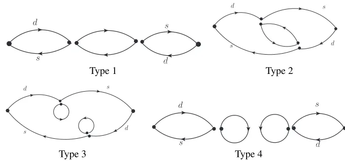
c (3 GeV) =750 MeV is unphysically light. The calculation has included all the contractions from Type 1 to Type 4 shown in Fig.8. Based on 120 configurations, the preliminary lattice result is given by∆MK=3.85(46)×10−12 MeV, which is consistent with the experimental value∆MK=3.483(6) ×10−12MeV [11]. However, since the calculation uses unphysical kinematics, this agreement could easily be fortuitous. Note that in the calculation of∆MK, the loop integral involves double Glashow-Iliopoulos-Maiani (GIM) cancellation [38] and thus, there is no short-distance divergence. On the other hand, the double GIM subtraction makes∆MKsignificantly rely on the charm quark mass. As a consequence, it is important to carry out the calculation at the physical charm quark mass.

d

s _d

s

Type 1

d

s d

s

Type 2

d s

s d

Type 3

d

s _d

s

Type 4

Figure 8.Four types of quark contractions for the calculation of∆MK.

are used to reduce the statistical uncertainty. Based on 59 configurations, the preliminary result of ∆MK=5.5(1.7) ×10−12 MeV is consistent with the experimental value. The project has planned to collect 160 measurements in total.

The status and prospects of the determination ofare updated by W. Lee in Refs. [44,45]. The estimate of is made using the FLAG value forBK, the angle-only-fit results for the Wolfenstein parameters and the CKM matrix elementVcb from exclusive or inclusive decays. The preliminary results foryield

∣∣SM=⎧⎪⎪⎨⎪⎪

⎩

1.66(17) ×10−3, using exclusiveVcb(Lattice QCD),

2.10(21) ×10−3, using inclusiveVcb(QCD sum rule). (37)

Here the exclusiveVcbis determined using the experimental measurements of ¯B→D∗ν¯and ¯B→Dν¯ together with the lattice QCD calculation for the corresponding hadronic matrix elements [10,46–

48]. The inclusive Vcb is determined using the inclusive decay process ¯B → Xcν¯ and QCD sum rules [49]. When using exclusiveVcb as input, there is a 3.3σdeviation between Standard Model value and experimental measurement∣∣exp =2.228(11) ×10−3. Besides,Vcbdominates the current 10% Standard Model uncertainty for. Therefore, it is important to have an accurate determination of Vcb. On the other hand, it is also important to compute the long-distance contribution toprecisely, whose size is expected to be a few percent but remains not well understood.

To calculate the long-distance contribution to, it is better to write the GIM cancellation by subtracting the charm quark propagator [40,41]

∑

q=u,c,t λq/p p2_+m2

q =

λu{ /p p2_+m2

u−

/

p p2_+m2

c} +

λt{ /p p2_+m2

t −

/

p p2_+m2

c}

. (38)

By doing so, the double GIM subtraction results in three terms in the effective Hamiltonian, with the coefficientsλ2u,λuλt andλ2t, respectively. Theλ2u term is irrelevant for. Theλ2t term is purely short-distance dominated. Therefore the only interesting term for lattice QCD calculation is theλuλt term.

d

s _d

s

Type 1

d

s d

s

Type 2

d s

s d

Type 3

d

s _d

s

Type 4

Figure 8.Four types of quark contractions for the calculation of∆MK.

are used to reduce the statistical uncertainty. Based on 59 configurations, the preliminary result of ∆MK =5.5(1.7) ×10−12 MeV is consistent with the experimental value. The project has planned to collect 160 measurements in total.

The status and prospects of the determination ofare updated by W. Lee in Refs. [44,45]. The estimate of is made using the FLAG value for BK, the angle-only-fit results for the Wolfenstein parameters and the CKM matrix elementVcb from exclusive or inclusive decays. The preliminary results foryield

∣∣SM=⎧⎪⎪⎨⎪⎪

⎩

1.66(17) ×10−3, using exclusiveVcb(Lattice QCD),

2.10(21) ×10−3, using inclusiveVcb(QCD sum rule). (37)

Here the exclusiveVcbis determined using the experimental measurements of ¯B→D∗ν¯and ¯B→Dν¯ together with the lattice QCD calculation for the corresponding hadronic matrix elements [10,46–

48]. The inclusiveVcb is determined using the inclusive decay process ¯B → Xc¯νand QCD sum rules [49]. When using exclusiveVcb as input, there is a 3.3σdeviation between Standard Model value and experimental measurement∣∣exp =2.228(11) ×10−3. Besides,Vcbdominates the current 10% Standard Model uncertainty for. Therefore, it is important to have an accurate determination of Vcb. On the other hand, it is also important to compute the long-distance contribution toprecisely, whose size is expected to be a few percent but remains not well understood.

To calculate the long-distance contribution to , it is better to write the GIM cancellation by subtracting the charm quark propagator [40,41]

∑

q=u,c,t λq/p p2_+m2

q =

λu{ p/ p2_+m2

u −

/

p p2_+m2

c} +

λt{ /p p2_+m2

t −

/

p p2_+m2

c}

. (38)

By doing so, the double GIM subtraction results in three terms in the effective Hamiltonian, with the coefficientsλ2u,λuλt andλ2t, respectively. Theλ2u term is irrelevant for. Theλ2t term is purely short-distance dominated. Therefore the only interesting term for lattice QCD calculation is theλuλt term.

In the lattice QCD calculation of λuλt contribution, the top quark field shall be integrated out, leaving a QCD penguin operator, shown in Fig.9. This QCD penguin operator can be neglected in

s d

s s

t W

g

=

⇒

s d

s s

=

⇒

d

s

s

s d

Type 5

Figure 9. QCD penguin operator and the origin of the Type 5 diagram for the calculation of the long-distance contribution to.

the calculation of∆MKas it carries a suppression factor ofλt/λu, but it is important for. The QCD penguin operator together with the current-current operator can form a new Type 5 diagram.

Without top quark in the lattice calculation, there is only one GIM subtraction and as a conse-quence the loop integral is logarithmic divergent. This divergence is cut offby an unphysical lattice scale, the inverse lattice spacing 1/a. One can define a bilocal operator in the RI-SMOM scheme by subtracting the unphysical short-distance contribution, and then match the bilocal operator in the RI-SMOM scheme to the one in the MS scheme using perturbation theory. More details on short-distance correction can be found in Refs. [40,50,51].

The calculation of is performed on a 243_{×64 lattice with domain wall fermion and Iwasaki} gauge action by RBC-UKQCD collaboration [40]. The inverse lattice spacing isa−1 _{is 1.78 GeV.} The pion mass is 339 MeV and the kaon mass 592 MeV. It uses 200 configurations and includes all Type 1-5 diagrams. In Table2the preliminary lattice results for long-distance contribution to,LD, are shown at various RI-SMOM scaleµRI ranging from 1.54 to 2.56 GeV. The µRI dependence is accounted for as a systematic uncertainty. AtµRI=2.11 GeV, the long-distance contribution to is about 5% when compared to the experimental value∣∣exp=2.228(11) ×10−3. To accurately estimate the long-distance contribution, the calculation needs to be performed at the physical kinematics.

Table 2.The long-distance contribution toat variousµRI, given in units of 10−3.

µRI 1.54 GeV 1.92 GeV 2.11 GeV 2.31 GeV 2.56 GeV LD 0.091(76) 0.104(76) 0.108(76) 0.111(77) 0.111(77)

3.3 Long-distance contributions to flavor changing process: rare kaon decays

Rare kaon decays have attracted increasing interest during the past few decades. As flavor changing neutral current processes, these decays are highly suppressed in the Standard Model and thus provide ideal probes for the observation of new physics effects. In this review, I will discuss the lattice QCD calculations of two classes of rare kaon decays:K→πν¯νandK→π+−[50–57].

TheK+ → π+ν¯νdecay is interesting because it receives the largest contribution from top quark loop and thus theoretically very clean. The required hadronic matrix elements can be obtained from leading order semi-leptonic K decays, such as K+ _{→ π}+_{eν, via isospin rotation. The remaining¯} long-distance contributions below the charm scale are expected to be a few percent. Though small, by including the long-distance contribution estimated from Ref. [58], the branching ratio Br(K+→π+ν¯ν) is enhanced by 6%, which is comparable to the 8% total Standard Model uncertainty [59]. The current known branching-ratio measurement [60]

¯

d

¯

s

u u

¯

u,¯c,t¯

e, µ, τ W W

ν

¯

ν

K+

π+

W-W

¯

d

¯

s

u u

W Z

¯

u,¯c,¯t ν

¯

ν

K+

π+

Z-exchange

Figure 10.Examples ofW-WandZ-exchange diagrams forK+→π+νν¯decay.

is a combined result based on the 7 events collected by BNL E787 [61–64] and its successor E949 [60,

65]. Its central value is almost twice of the Standard Model prediction [59]

Br(K+→π+ν¯ν)SM=9.11±0.72×10−11, (40)

but with a 60-70% uncertainty it is still consistent with Standard Model.

The new experiment, NA62 in CERN [66], aims at an observation ofO(100)events and a 10%-precision measurement of Br(K+→π+ν¯ν). The status reported at the Flavor physics and CP violation workshop (FPCP 2017) is that the detector installation is completed in September 2016. 5% of the 2016 data has been analyzed but no event is found yet. If using full 2016 data, thenO(1)events are expected to be found. Considering the fact that the Standard Model predictions will be confronted with the new experiment soon, a lattice QCD calculation of the long-distance contribution toK+→π+νν¯ is timely.

There are two classes of diagrams, which contribute toK+ → π+ν¯νdecays, called asW-W and Z-exchange diagrams. In theW-W diagrams the second-order weak transition proceeds through the exchange of twoW-bosons, while for theZ-exchange diagrams the decay occurs through the exchange of oneW-boson and oneZ-boson. Examples of both classes of diagrams are illustrated in Fig.10.

In a lattice QCD calculation, theW andZ-boson have been integrated out, leaving two effective four-fermion local operators. The matrix element of the time-integrated bilocal operator is evaluated in Euclidean space. This matrix element can be related to the second-order amplitude of interest if a sum over intermediate states is inserted and the integration over Euclidean time performed:

∫_−TTdt⟨π+νν∣T{HA(t)HB(0)} ∣K+⟩

= ∑

n

⎧⎪⎪ ⎨⎪⎪ ⎩

⟨π+νν∣HA∣n⟩⟨n∣HB∣K+⟩

En−EK + ⟨

π+νν∣HB∣n⟩⟨n∣HA∣K+⟩ En−EK

⎫⎪⎪ ⎬⎪⎪ ⎭(1−e

(EK−En)T)_,(41)

whereHA/B(t)stands for the two four-fermion operators, with the spatial variables integrated over space. The unphysical e(EK−En)T _{terms in the second line of this equation vanish for largeT for} intermediate states more energetic than the kaon. However, these terms grow exponentially with increasing integration range ifEn < EK and must be removed from lattice calculation. When the intermediate state involves multiple particles, the branch-cut integral in the infinite volume is replaced by a discrete state summation in the finite volume. It could cause potentially large finite-volume effects whenEn→MK, which need to be corrected following Ref. [67].