c
Owned by the authors, published by EDP Sciences, 2015
Numerical simulation of large deformations of amorphous polymer with
finite element method: Application to normal impact test
C.A. Bernard1,a, J.P.M. Correia1, N. Bahlouli1, and S. Ahzi1,2
1University of Strasbourg/CNRS, ICUBE Laboratory, 2 rue Boussingault, 67000 Strasbourg, France 2Qatar Environment and Energy Research Institute, Qatar Foundation, PO Box 5825, Doha, Qatar
Abstract. During the last decades, the part of polymeric materials considerably increased in automotive and packaging applications. However, their mechanical behaviour is difficult to predict due to a strong sensitivity to the strain rate and the temperature. Numerous theories and models were developed in order to understand and model their complex mechanical behaviour. The one proposed by Richeton et al. [Int. J. Solids Struct. 44, 7938 (2007)] seems particularly suitable since several material parameters possess a strain rate and temperature sensitivity. The aim of this study is to implement the proposed constitutive model in a commercial finite element software by writing a user material subroutine. The implementation of the model was verified on a compressive test. Next a normal impact test was simulated in order to validate the predictive capabilities of the model. A good agreement is found between the FE predictions and the experimental results taken from the literature.
1. Introduction
Amorphous polymeric materials exhibit interesting me-chanical and physical properties. Thus, polymers are widely used for large-strain applications in the automotive or packaging industries. Below the glass transition temper-ature, amorphous polymers exhibit a complex behaviour which is strain rate and temperature dependent [1,2]. According to the literature, the initial elastic linear response is followed by a viscoelastic response which ends at the yield point. Then, a viscoplastic response takes place characterized by a strain softening followed by a large strain hardening.
Nowadays, finite element (FE) simulations are widely used to improve geometry of structures. However, the mechanical behaviour of polymeric materials needs to be correctly reproduced. During the last decades, numerous models based on physical considerations were developed [3–5] in order to simulate the thermo-mechanical behaviour of amorphous polymer in the glassy region. A model particularly suitable is the one developed by Richeton et al. [4]. In the model, the elastic modulus and yield strength are strain rate and temperature dependent. They also proposed a thermally activated flow rule based on the cooperative model initially presented in the work of Fotheringham and Cherry [6]. These constitutive equations [4] allow reproducing the stress-strain curves of amorphous polymers over a wide range of strain rate and of temperature.
The aim of this study is to implement the constitutive equations proposed by Richeton et al. [4] in the com-mercial FE code ABAQUS/Explicit through a VUMAT subroutine. Firstly, the model formulation is detailed. Then, the integration algorithm is presented and validation
aCorresponding author:
tests at constant strain rate are performed in order to verify the correct implementation of the constitutive equation. Finally, FE simulations of an impact test were carried out. A good agreement is observed between the FE predictions and the experimental results [7].
2. Constitutive equations
The three-dimensional constitutive model used to describe the mechanical behaviour of amorphous polymers under finite strain is based on the work of Richeton et al. [4]. Ac-cording to the kinematics of finite strain, the deformation gradient tensor F is multiplicatively decomposed into an elastic, thermal and plastic components:
F=FeFt hpwith Ft hp =Ft hFp (1) with Fp the plastic deformation gradient defined from the reference configuration to the first relaxed configuration, the plastic deformation gradient defined from the reference configuration to the first relaxed configuration, Ft h the
thermal deformation gradient defined from the first configuration to the second relaxed configuration and Fe the elastic deformation gradient defined from the second relaxed configuration to the current configuration. The polar decomposition of F, Feand Fpare given by:
Fi =RiUi=ViRi with i =e,p (2) with R the rotation tensor, U the right stretch tensor and V the left stretch tensor. The velocity gradient tensor L is given by:
L=FF˙ −1. (3)
Incorporating Eq. (1) into Eq. (3), one obtains:
with
Le=F˙eFe−1,Lt h =F˙t hFt h−1,Lp=F˙pFp−1. (5) The velocity gradient tensor L can be decomposed as follows:
L=D+W (6)
where D is the rate of deformation tensor (symmetric part) and W the spin tensor (skew-symmetric part). According to Eq. (6), the elastic, thermal and plastic velocity gradients are given by:
Le=De+We,Lt h =Dt h +Wt h,Lp =Dp+Wp. (7) In the following, two basic assumptions are made. Firstly, we assumed that the plastic flow is incompressible. Thus,
det Fp=1,det Ft h=1,det Ft hp=1. (8) We also assumed that the thermoplastic flow is irrotational. By consequence,
Wp =0,Wt h =0,Wt hp=0. (9) In this work, the elastic behaviour of amorphous polymers is assumed to be linear isotropic and can be modelled using the classical Hooke’s law. The Cauchy stress tensor T is defined by:
T= 1
det FeC
e
ln Ve (10)
with ln Ve the Hencky strain and Ce the fourth order stiffness tensor defined by:
Cei j kl =
E 1+ν
1
2δi kδjl+δilδj k+ ν 1−2νδi jδkl
(11)
with E the Young’s modulus, ν the Poisson’s ratio and δ the Kronecker-delta symbol. The strain rate and temperature dependence of the Young’s modulus is given by Richeton et al. [8]:
E(θ,ε˙)= (E1(˙ε)−E2(˙ε)) exp
−
θ Tβ(˙ε)
m1
+ (E2(˙ε)−E3(˙ε)) exp
−
θ
Tg(˙ε) m2
+ E3(˙ε) exp
−
θ
Tf(˙ε) m3
(12)
where θ is the absolute temperature, ˙ε is the effective strain rate, Tβ is theβ-transition temperature, Tg is the
glass transition temperature, Tf is the flow temperature,
Eiare the instantaneous stiffness of the material measured
by DMA at the beginning of each transition region (glassy, glass transition and rubbery region) and mi
the Weibull moduli corresponding to the statistics of bond breakage. The different instantaneous moduli and
transition temperatures are strain rate dependent and follow the expressions:
Ei(˙ε)=E r e f i
1+silog
˙ ε/ε˙r e f 1
Tβ(˙ε) = 1 Tβr e f +
R
Hβ ln
˙ εr e f/ε˙
Tg(˙ε)=Tgr e f −
c2log(ε˙r e f/ε)˙ c1+log(ε˙r e f/ε)˙
Tf(˙ε)=T r e f f
1+0.01 logε/˙ ε˙r e f
(13)
with Eir e f, T r e f
β , Tgr e f, T r e f
f the instantaneous moduli and
the transition temperatures at the chosen reference strain rate ˙εr e f, sithe strain rate sensitivity parameters,Hβ the
β-activation energy, R the ideal gas constant and c1, c2
the WLF parameters [9]. According to literature [10–12], the Poisson’s ratio of amorphous polymers is strain rate and temperature dependent in the glass transition region. In this region, the Poisson’s ratio sharply increases and achieves a value close to the Poisson’s ratio of a rubbery material. In order to take into account this phenomenon, the following phenomenological model is proposed by Bernard et al. [13]:
ν(θ,ε˙)=
ν0+(νc−ν0) exp
−θ−(Tg(˙ε)+θ) 2
2ω2
ifθ <Tg +θ
νc
ifθ≥Tg+θ
(14)
whereν0andνcare respectively the Poisson’s ratio values
at the beginning and at the end of the glass transition region,θ is related to the half of the temperature range across which the glass transition occurs and where 2ω= ω1/
√
ln 4 withω1 the full width at half maximum of the
Gaussian function.
The end of the elastic behaviour is characterized by the yield point. The yield strength is modelled with the equations proposed by Richeton et al. [14]. Below the glass transition temperature Tg, the yield strengthτyis given by:
τy=τi(θ)+
2kθ V sinh −1 γ˙ θ <Tg
˙ γ0exp
−Hβ
Rθ
1/n
(15)
withτi(θ) the evolving internal shear stress at the absolute
temperatureθ, k the Bolzmann constant, V the activation volume, ˙γ the effective shear strain rate, ˙γ0 a
pre-exponential shear strain rate constant and n describes the cooperative character of the yield strength. At the yield point, the internal stress is expressed as:
τiy(θ)=τi(0)−mθ +αpwith P=−
1
3tr(T) (16) withτi(0) the internal stress at 0 K, m a material constant,
αp a pressure sensitivity parameter and P the hydrostatic
pressure.
introduced the expression of the thermoplastic strain rate tensor Dt hpas:
Dt hp =Dp +β(θ) ˙θI (17) with β(θ) the thermal expansion coefficient equal to β(298 K ) ifθ <Tg(in agreement with [15,16]) and I the
identity tensor. The plastic strain rate tensor Dp is given by:
Dp = γ˙
p √
2τT
∗
(18) where T∗ is the deviatoric part of the driving stress tensor T∗expressed in the isothermally unloading configuration, τ is the effective shear stress defined by:
τ =
1 2T
∗ : T∗
1/2
(19) and ˙εp is the effective plastic shear rate. Below Tg, the
effective plastic shear rate is expressed as: ˙
γp =
˙ γ0exp
−Hβ
Rθ
sinhn
(τ −τi)V
2kθ
(20) where the material constants are the same as in Eq. (15). The strain softening is modelled by the evolution of the internal stressτi. This stress evolves significantly from its
initial valueτiy. In agreement with Boyce et al. [17], the
evolution ofτifollows the phenomenological law given by:
˙ τi =h
1− τi τps
˙ γp
(21) with h the softening slope andτpsthe stress referring to the
preferred structural state of the material. In Eqs. (18) and (19), the deviatoric part of the driving stress tensor appears. It is expressed in the isothermally unloading configuration. In the intermediate configuration, the driving stress tensor is given by:
T∗=ReTTRe−B (22)
with B the backstress tensor which allow to take into account the important strain hardening of the material. In [4], the backstress tensor B is assumed to be coaxial to the plastic stretch tensor Vp. In accordance with Arruda and Boyce [18], the principal components of B are given by:
Bi =CR(θ) √
N (θ)
3 L
−1 λchai n √
N (θ)
λ2
i −λ2chai n
λchai n
for i =1,2,3 (23)
with CRthe rubbery modulus, N the number of rigid chain
links between entanglements, L−1 the inverse Langevin function that is estimated with the Pad´e approximation proposed by Cohen [19],λi are the principal components
of Vp, andλchai nis the plastic stretch on a chain (or called
network locking stretch):
λchai n =
λ2
1+λ22+λ23
3 · (24)
According to Richeton et al. [4], CRand N are temperature
dependent parameters. More details on the model can be found in [4].
3. Computational procedure
The constitutive model presented above was implemented into the FE code ABAQUS/Explicit through a user material subroutine VUMAT [20].
At each step time and for each integration point of the elements, the FE code provides the Cauchy stress tensor T and the user-defined state variables defined at time t, and the time incrementt . In addition, the FE code estimates the strain increment tensorε, the deformation gradient tensor F, the temperatureθ and the right stretch tensor U at time t +t . At the end of each time increment, the user needs to return to ABAQUS/Explicit the updated values of Cauchy stress tensor T and of state variables.
At the beginning of the computation, at time t =0, the material is assumed to have an elastic behaviour (Fp = Ft h =Ft hp=I) and have an initial temperatureθ. In small strain, amorphous polymers exhibit an elastic behaviour. Thus, the elastic deformation gradient tensor Fe equals the deformation gradient tensor F. After performing the polar decomposition on Fe, the Cauchy stress tensor T
is computed at time t+t using Eq. (10). When the effective stressτ reaches the yield strengthτy, the plastic
and thermal deformation gradient tensors deviate from the identity tensor. These tensors have to be derived from the viscoplastic flow rules, Eqs. (17)–(24). In order to update the Cauchy stress tensor Tt+t, an implicit time
computation scheme was used. More details about the computational procedure could be found in [13].
4. Computational test
To check the implementation of the constitutive model, preliminary FE simulations were performed. The material is a polycarbonate (PC) studied by Richeton et al. [4]. The material was tested in uniaxial compression at 25◦C and at a constant strain rate of 10 s−1. The material parameters can be found in the work of Richeton et al. [4].
The validation tests were performed on a square firstly meshed with one element CPE4R (continuum plane strain element with reduced integration) and next divided into 10×10 elements. The meshed square was subjected to a compression test with a constant strain rate under isothermal and adiabatic conditions.
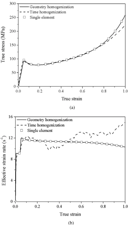
A good agreement is obtained between the numerical predictions found in [4] and the FE predictions with one element. However, for a large number of elements, a distortion of the mesh is noticed as illustrated by Fig.1(a). This phenomenon is due to an instability of the effective strain rate, ˙εt+t that leads to a non-convergence of
the problem as shown in Fig. 1(b) for three different elements. Thus, two averaging techniques are investigated in order to stabilize the effective strain rate: geometry homogenization and time homogenization.
4.1. Geometry homogenization
(a)
(b)
Figure 1. (a) Deformed shape of a square geometry meshed with
10×10 elements tested in uniaxial compression at 25◦C and at 10 s−1. (b) Strain rate-time curve for three elements of the mesh.
increment and for all the elements with the same abscissa, an average effective strain rate is computed. Thus, the geometry averaged effective strain rate ˙εH G is defined by:
˙ εH G =
1 ne
ne
i=1
˙
εi (25)
with nethe number of element with the same abscissa and
˙
εithe effective strain rate for the element i .
4.2. Time homogenization
The time increment averaging method is based on the assumption that the effective strain rate evolves smoothly. The time increment homogenization method consists in averaging the effective strain rate on a given interval of time for each element. Thus, the time averaged effective
(a)
(b)
Figure 2. FE predictions of uniaxial compressive test at a
constant strain of 10 s−1 for an unique element and 10×
10 elements: (a) stress-strain curve and (b) effective strain rate.
strain rate ˙εH T is defined by:
˙ εtN
H T = N−1
j=i
˙ εtj
H T∗tj
+ε˙tN∗tN
N
j=i
tj
(26)
where tN−tirepresents the interval of time where the time
homogenization is done.
4.3. Results and discussion
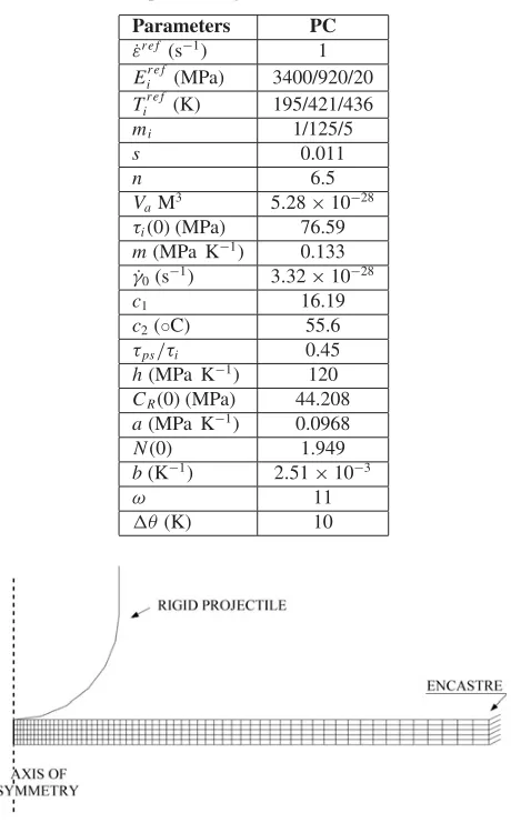
Table 1. Material parameters of the proposed model for PC
identified on the experiments given in Ames et al. [7].
Parameters PC
˙
εr e f (s−1) 1
Eir e f (MPa) 3400/920/20 Tir e f (K) 195/421/436
mi 1/125/5
s 0.011
n 6.5
VaM3 5.28×10⁻²⁸
τi(0) (MPa) 76.59
m (MPa K−1) 0.133
˙
γ0(s−1) 3.32×10⁻²⁸
c1 16.19
c2(◦C) 55.6
τps/τi 0.45
h (MPa K−1) 120
CR(0) (MPa) 44.208
a (MPa K−1) 0.0968
N (0) 1.949
b (K−1) 2.51×10⁻³
ω 11
θ(K) 10
Figure 3. FE mesh used in the thermo-mechanically coupled
analysis of normal impact test.
contrary to the strain rate predicted by the geometry homogenization. The two homogenization techniques gave good results. In spite of some instabilities of the effective strain rate for the time homogenization method, this technique is more suitable since it is easier to use.
5. Normal impact test
A normal impact test was modelled and simulated with ABAQUS/Explicit. This impact test and the experimental results are taken from the work of Ames et al. [7]. In this test a circular plate of PC is clamped and is impacted by a spherical-tipped cylindrical projectile. The mechanical behaviour of the PC was described with the constitutive model presented above. Some material properties were determined by Ames et al. [7]. The other parameters were identified from stress-strain curves presented in [7] and are listed in Table1.
ABAQUS/Explicit code was used for the FE simula-tion using the VUMAT subroutine previously validated. In order to reduce the computation time, the axi-symmetry of the problem was used and thus only one slice of the
Figure 4. Reaction force versus time response for the projectile.
Figure 5. Comparison between experimental and numerically
predicted section profiles.
Figure 6. Influence of the projectile diameter size in the section
profiles.
geometry was meshed. The PC plate has an initial radius of 101.6 mm and a thickness of 5.334 mm. The projectile, with a mass of 80 kg and a radius of 22.5 mm, impacts the plate at a velocity of 3.6 ms−1.
The PC plate was meshed with 300 elements CAX4RT (4-node bilinear displacement and temperature, reduced integration with hourglass control element). All the nodal displacements were constrained on the right side of PC plate. The geometry of the test and of the mesh are presented in Fig.3. The contact between the projectile and the plate is assumed frictionless.
However, in Fig.5, a discrepancy between the profile shapes is observed under the projectile. In order to analyse the effect of projectile geometry, FE simulations with three different projectile diameters were carried out. The predicted results are compared with the experimental ones measured by Ames et al. [7] in Fig. 6. We can note that the best fit is obtained with a projectile diameter of 17.5 mm.
6. Conclusion
An elastic-viscoplastic model has been implemented in the commercial FE code ABAQUS/Explicit, via a VUMAT subroutine, in order to simulate the mechanical response of amorphous polymers. The numerical implementation of the constitutive model was first validated for a unique and several elements in plane strain conditions. In order to stabilize the mechanical response, homogenization techniques for averaging the strain rate have been proposed. Both homogenization methods gave good results. A normal impact test on a PC plate was modelled and simulated. A good agreement was found between the numerical prediction and the experimental results taken from the literature [7].
References
[1] M.R. Boumbimba, E. Hablot, K. Wang, N. Bahlouli, S. Ahzi, L. Av´erous, Compos. Sci. Technol. 71, 674 (2011)
[2] K. Wang, F. Addiego, N. Bahlouli, S. Ahzi, Y. R´emond, V. Toniazzo, Compos. Sci. Technol. 95, 89 (2014)
[3] E.M. Arruda, M.C. Boyce, R. Jayachandran, Mech. Mater. 19, 193 (1995)
[4] J. Richeton, S. Ahzi, K.S. Vecchio, F.C. Jiang, A. Makradi, Int. J. Solids Struct. 44, 7938 (2007) [5] L. Anand, N.M. Ames, V. Srivastava, S.A. Chester,
Int. J. Plasticity 25, 1474 (2009)
[6] D.G. Fotheringham, B.W. Cherry, J. Mater. Sci. 13, 951 (1978)
[7] N.M. Ames, V. Srivastava, S.A. Chester, L. Anand, Int. J. Plasticity 25, 1495 (2009)
[8] J. Richeton, G. Schlatter, K.S. Vecchio, Y. R´emond, S. Ahzi, Polymer 46, 8194 (2005)
[9] M.L. Williams, R.F. Landel, J.D. Ferry, J. Am. Chem.l Soc. 77, 3701 (1955)
[10] G.N. Greaves, A.L. Greer, R.S. Lakes, T. Rouxel, Nat. Mater. 10, 823 (2011)
[11] P. H. Mott, J. R. Dorgan, C. M. Roland, J. Sound Vib. 312, 572 (2008)
[12] S. Pandini, A. Pegoretti, eXPRESS Polym. Letters 5, 685 (2011)
[13] C.A. Bernard, J.P.M. Correia, S. Ahzi, N. Bahlouli, (in preparation) (2015)
[14] J. Richeton, S. Ahzi, L. Daridon, Y. R´emond, Polymer 46, 6035 (2005)
[15] J. Bicerano, Prediction of polymer properties, (CRC Press, 2002)
[16] D.W. van Krevelen, K. te Nijenhuis, Properties of polymers : their correlation with chemical structure; their numerical estimation and prediction from additive group contributions, (Elsevier Science & Technology Books, 2009)
[17] M.C. Boyce, D.M. Parks, A.S. Argon, Mech. Mater. 7, 15 (1988)
[18] E. M. Arruda, M.C. Boyce, J. Mech. Phys. Solids 41, 389 (1993)