Application of Passivity to Adaptive Control
Compensation Systems
V.Srinivasan, T.Saravanan
Assistant Professor, Dept of ETC, Bharath University, Chennai, Chennai, Tamil Nadu, India
Professor, Dept of ETC, Bharath University, Chennai, Tamil Nadu, India
ABSTRACT: In this paper the model reference adaptive system (MRAS) is considered. The feedforward gain adjustment is done by using adaptive technique and feedforward gain compensation by passivity-based technique is presented. The adaptation of feedforward gain is considered by using MIT rule and the effect of variation of parameter values and adaptation gain on the response of the system is simulated. But to achieve more stable system, Lyapunov stability theorem is used for parameter adjustment. It has been shown that the adjustment rule guarantees that error goes to zero. Finally input-output stability theorem is used to construct adjustment rules for the adaptive system. The passivity theorem is applied to construct adjustment laws. The compensating network is introduced so that the transfer function relating the error is strictly positive real (SPR). The compensator is designed by using Kalman – Yakubovich (KY) Lemma. Simulation results are furnished after implementing the adaptive techniques. Algorithm for the design of compensator using KY Lemma is also presented.
KEYWORDS: Feedforward gain; Parameter adjustment; Passivity; Strictly positive real; KY lemma;MIT rule.
1. INTRODUCTION
The model reference adaptive control (MRAC) technique has been a popular approach to the control systems operating in the presence of parameter and environmental variations. The MRAC system was first designed by the performances index minimization method proposed by Whitaker of MIT Instrumentation Laboratory and since then has been referred as the MIT rule. This rule has been very popular because of its simplicity in practical implementation. In this technique output rate of convergence depend upon the adaptation gain [1-3].
The other approach to adaptation is based on Lyapunov’s second method. The adaptive rule is obtained by selecting the design equations to satisfy conditions derived from Lyapunov’s second method [4], so that the system stability is guaranteed for all inputs. The quadratic Lyapunov function was employed by Parks to redesign systems formerly designed by MIT rule. The main disadvantage of Lyapunov method is that the entire state vector must be available for measurement, which is not often possible [4,5].
The concept of positive realness plays a central role in stability theory in general and in many of the stability proofs of adaptive systems [1,6]. The definition of positive real (PR) function of a complex variable s arises in circuit theory. Brune showed that the driving point impedance of a passive network is rational and positive real. If the network is dissipative, due to the presence of resistors, the driving point impedance is strictly positive real. In other words, a PR and SPR rational function can be realized as the driving point impedance of passive network. In this context KY lemma finds applications in adaptive control theory [6].
2.1 MIT Rule
Consider a closed loop system in which a controller has one adjustable parameterθ. A model whose output is ym specifies the desired closed loop response. Let e be the error between the output y of the closed loop system and the output ym of the model. To adjust the parameters in such way that the loss function J(θ) = ½ e2 is minimized. To make
J small, it is possible to change the direction of the negative gradient of J, i.e.
dθ
= −γ
∂J
= −γe
∂e
(1)
dt ∂θ ∂θ
This is the well-known MIT rule. The partial derivative ∂e/∂θ, which is called the sensitivity derivative of the system and tells about the influence of error due to parameter variation.
2.2 Statement of the Problem
The problem under consideration is to adjust feedforward gain. In this problem it is assumed that the process is linear with the transfer function kG(s), where G(s) is known and k is unknown parameter. The design problem is to find a feedforward controller that gives a system with the transfer function Gm(s) = k0G(s), where k0 is given constant. With the feedforward controller u=θuc. Where u is the control signal and uc is the command signal and assuming parameter
θ = k0/k.
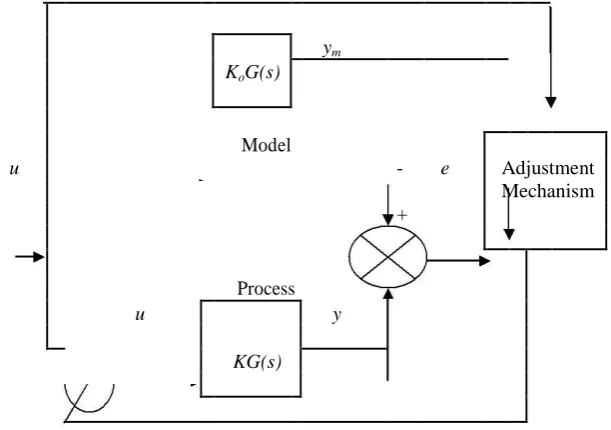
The problem is described by following block diagram.
ym
KoG(s)
u Model
- e
Adjustment + Mechanism u Process y KG(s)
Fig. 1. Block Diagram of Feedforward Gain Adaptation Problem
Now using the MIT rule to obtain a method for adjusting the parameter θ when k is not known. From Fig. 1
y = kG(d/dt) θ uc, (2)
ym = koG(d/dt) uc (3)
The error is –
e = y – ym = kG(d/dt) θuc – koG(d/dt) uc
= kG(d/dt)( θ - θ0
) uc (4)
Where d/dt is differential operator and θ0 = ko /k
but from equation (3), G(d/dt)u c =
y m
, therefore Equation 5 becomes
k 0 ∂e
=
k
y m (6)
∂θ k 0
As per the MIT rule Equation 1 the adaptation law can be written as -
dθ = −γ'
k
ym e = −γ ym e (7)
dt k0
after integrting both sides of Equation 7,
θ(t)=-γ ym∫t e(s)ds (8)
where γ = γ'
k
, Equation 8 gives the law for adjusting the parameter.
k0
2.3 Simulation of the System
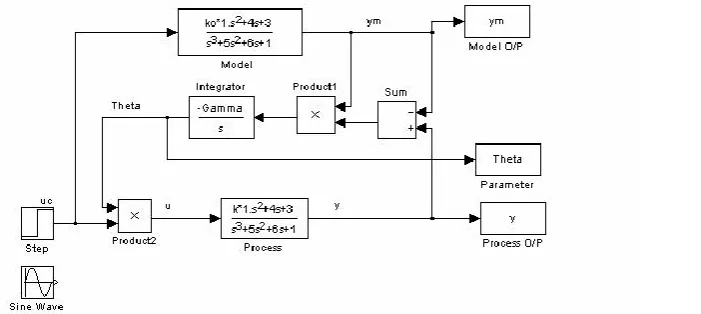
The adjustment mechanism of Fig. 1 can be thought of as composed of three parts – a linear filter for computing the sensitivity derivative from inputs and outputs, a multiplier, and an integrator.
Now by using MATLAB Simulink for simulation of the block diagram shown in Fig. 1 and implementing the feedforward gain adjustment law obtained by MIT rule Equation 8. For this purpose let us consider the transfer function
G(s)=
s 2+4s + 3
(9)
s3 +5s2 + 6s +1
The simulation block diagram is shown in following Fig. 2
The input uc is chosen as unit step or as sinusoidal of frequency 1 rad/sec selecting from source library. The parameters k, ko are chosen as k = 1, and ko = 2. The results of simulation are given by Fig. 3 where y, ym,θ, and e are shown for different γ values, such as γ = 0.5 and 0.75.
a) Step Response for Adaptation gain =0.5 and 0.75 b)Sinusoidal Response for Adaptation gain =0.5 and 0.75 Fig. 3
Simulation of MRAS for adjusting a feedforward gain
From Fig. 3 it has been noted that, for both step and sinusoidal the response of the system depends on the adaptation gain. The convergence rate depends on the value of γ. For small value of γ convergence rate decreases and for high value of gamma convergence rate increases. But there is no guarantee of the system stability in this adaptation technique.
III. ADAPTATION BY LYAPUNOV THEOREM
The first step in the stability approach to adaptive system design is the choice of the adaptive law for adjusting the control parameters to assure stability. An alternative method for adaptation of MRAS based on Lyapunov’s second method is suggested and here it is applied to the problem under consideration.
3.1 Lyapunov Teory
The problem of stability in previous method is considerably improved in this method. Now Lyapunov’s stability theorem is used to construct algorithm for adjusting parameters in adaptive system. For this let us consider a differential Equation for error, e = y – ym. This differential Equation contains the adjustable parameters. Then it is required to choose a suitable Lyapunov function and an adaptation mechanism so that the error goes to zero.
The error is given by Equation 4 and now using Lyapunov theorem [1,4,7], first consider the Equation of the system as –
.
e = Ae + k (θ −θ 0)uc (10)
writing state equations by considerin g the relation between th e parameter θ and error e then,
dx
= Ax + b(θ −θ0 )uc
dt
e = Cx (11) .
= Ax is asymptotic ally stable, there exist positive definite If the homogeneou s system x
matrices P and Q such that A TP + PA = −Q (12) Now choosing the Lyapunov function as -
V = 1
(γ xT Px +(θ −θ 0)2)
(13)
2
The time derivative of V is given by -
dV
γ
T
T dx
0
dθ
dt 2 dt dt dt
by using equation 10, equation 13 becomes -
dV γ
x T
Qx +(θ
0 dθ T
= − −θ ) + γucB Px (15)
dt 2 dt
therefore from equation (14) the parameter adjustment law is chosen to be -
dθ
= −γucB T
Px
(16)
dt
From Equation 16, it is to be noted that, the derivative of Lyapunov function will be negative
as long as x ≠ 0. The state vector x and the error e = Cx will go to zero as t goes to ∞. But parameter error (θ −θ0 ) will
not necessarily go to zero. In this technique the restriction is that it requires that all state variables are known. A
parameter adjustment law that uses output feedback can be obtained if Lyapunov function can be chosen such that BT
P =C, where C is the output matrix of the system. Therefore,
BT Px = Cx = e, and the adjustment law becomes
dθ
= −γuce (17)
dt
3.2 Simulation of the System
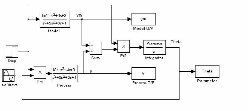
The control law obtained above Equation 17 is used to construct the adjustment mechanism of Fig. 1 and modified by block diagram as shown in Fig. 4, a simulation diagram using MATLAB Simulink. Here again the input signal uc is step and sinusoidal are applied to the system and simulation results are shown in Fig. 5.
In this section it has been shown that it is possible to construct parameter adjustment rules based on Lyapunov’s stability theory. The adjustment rules obtained in this way guarantee that the error goes to zero, but it cannot be asserted that the parameters converge to their correct values. Therefore some advanced technique like passivity is used to construct adjustment rules for the adaptive system.
a) Step Response for Adaptation gain =0.5 and 0.75 b)Sinusoidal Response for Adaptation gain =0.5 and 0.75
Fig. 5 Simulation of MRAS for adjusting a feedforward gain using Lyapunov Theory
IV. ADAPTATION BY PASSIVITY THEOREM
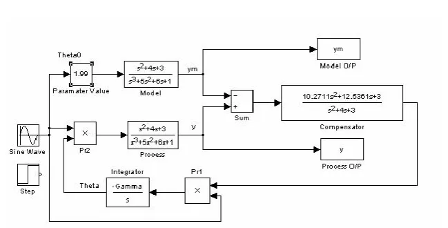
The problem of feedforward gain compensation is the main objective of this paper. In this section compensation obtained an adjustment rules based on passivity theorem. The same problem was treated in Section 2 with Lyapunov’s stability theory and obtained parameter adjustment law described by Equation 17. According to passivity theorem the adaptive system will be stable if the transfer function G(s) is SPR. This condition indicates that the result is related to passivity theory.
4.1 Application of Passivity to Adaptive Control
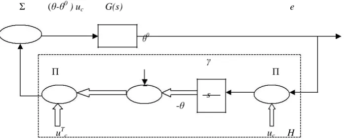
The passivity theorem [1,6,7] along with small gain theorem is used to derive stability results for the system under consideration Fig. 1. Fig. 6 shows a linear time invariant system described by G(s) and that corresponds to the plat together with a fixed controller, while the feedback system H corresponds to the mechanism generating the parameter error, θ and the corresponding control input (θ – θ0)uc. Thus passivity theorem [1,7] is applied directly to such systems to prove L2 – Stability if G(s) is strictly passive and H is passive.
Σ (θ-θ0) uc G(s) e
θ0
Π
Σ
γ
Π
s
-θ
uTc uc H
Fig. 6 Block diagram for the system with adjustable feedforward gain when using the control law of Equation 17
Fig. 7 A Stable Parameter Adjustment Law by Passivity and KY Lemma
4.2 Algorithm based on KY Lemma for Designing Compensator
Step - I: By using KYP Lemma G(s) = B(s)/A(s) Finding polynomial C(s) such that C(s)/A(s) is SPR
Canonical realization of 1/A(s) is obtained by using tf2ss command of control system toolbox Step - II: Choosing a symmetric positive definite matrix Q and finding matrix P by using lyap command.
Step - III: The coefficients of a C polynomial such that C(s)/A(s) is SPR are then the first row of the P Matrix. i.e. C = P(1,:)
Therefore numerator polynomial of Gc= C and denominator polynomial of Gc is polynomial of B(s).
a) Step Response for Adaptation Gain = 0.5 and 0.75 b) Sinusoidal Response for Adaptation Gain = 0.5 and 0.75 Fig. 8 Simulation of MRAS for a feedforward gain Compensation using KY Lemma
V. CONCLUSION
The problem in which the system under consideration Fig. 1, where adjustment mechanism replaced by MIT rule Equation 8 was performed well for the smaller adaptation gain but stability is disturbed for slightly increase in the γ value. Therefore the allowable range of the Gamma depends on the magnitude of the reference signal. Consequently it is not possible to give fixed limits which guarantee stability. Thus the MIT rule based adaptive systems are said to be closed loop unstable systems.
Adaptation based on Lyapunov’s direct method guarantees the stability for all kinds of inputs and allows high gains in the adaptive loops i.e. adaptation gain, γ. From Fig. 5 it has been seen that the stability of the system is asymptotic for the chosen k, k0andγ values.
1. Karl J. Åström, Björn Wittenmark, Adaptive Control, Second Edition, Pearson Education Asia, 1995.
2. Bhat V., "A close-up on obturators using magnets: Part I - Magnets in dentistry", Journal of Indian Prosthodontist Society, ISSN :
0972-4052 , 5(3) (2005) pp.114-118.
3. Karl J. Åström, “Theory and Applications of Adaptive Control – A Survey”, Automatica,Vol. 19, pp 471 – 486, Sept 1983
4. Nagarajan C., Madheswaran M., "Stability analysis of series parallel resonant converter with fuzzy logic controller using state space techniques", Electric Power Components and Systems, ISSN : 1532-5008, 39(8) (2011) pp.780-793.
5. Madan M. Gupta, Adaptive Methods for Control Systems Design: An Overview, Adaptive Methods for Control System Design, IEEE Press selected reprint series, 1986, pp. 1-2.
6. Khanaa V., Thooyamani K.P., Saravanan T., "Simulation of an all optical full adder using optical switch", Indian Journal of Science and Technology, ISSN : 0974-6846, 6(S6)(2013) pp.4733-4736.
7. Patrick C. Parks, “Liapunov Redesign of Model Reference Adaptive Control System”,
IEEE Transaction on Automatic Control, Vol. AC – 11, pp. 362 – 367, July 1966.
8. Madhubala V., Subhashree A.R., Shanthi B., "Serum carbohydrate deficient transferrin as a sensitive marker in diagnosing alcohol abuse: A
case - Control study", Journal of Clinical and Diagnostic Research, ISSN : 0973 - 709X, 7(2) (2013) pp.197-200.
9. Chang-Chien Hang, Patrick C. Parks, “Comparative Studies of Model Reference Adaptive Control Systems”, IEEE Transaction on
Automatic Control, Vol. AC – 18, pp.419-428, Oct. 1973.
10. Shanthi B., Revathy C., Devi A.J.M., Parameshwari P.J., Stephen T., "Serum 25(OH)D and type 2 diabetes mellitus", Journal of Clinical
and Diagnostic Research, ISSN : 0973 - 709X, 6(5) (2012) pp.774-776.
11. Shankar Sastry, Mark Bodson, “Adaptive Control Stability, Convergence andRobustness”, Prentice Hall of India Private Ltd., 1989. 12. Kumpati S. Narendra, Anuradha M. Annaswamy, Stable Adaptive Systems, Prentice Hall Information and System Science Series,
Englewood Cliffs, New Jersey, 1989.
13. B Karthik, TVU Kirankumar, MS Raj, E BharathKumaran,Simulation and Implementation of Speech Compression Algorithm in VLSI, Middle-East Journal of Scientific Research 20 (9), PP 1091-1092, 2013.
14. A.Geetha, Face Recognition Using OPENCL, International Journal of Advanced Research in Electrical, Electronics and Instrumentation Engineering , ISSN (Print) : 2320 – 3765, pp- 7148-7151, Vol. 3, Issue 2, Febuary 2014.
15. A.Geetha, Universal Asynchronous Receiver / Transmitter (UART) Design for Hand Held Mobile Devices, International Journal of Advanced Research in Electrical, Electronics and Instrumentation Engineering, ISSN: 2231-5381, pp 25-26, Volume 3 Issue 1 No1 – January 2012. 16. D.Sridhar raja, Comparison of UWB Band pass filter and EBG embedded UWB Band pass filter, International Journal of Advanced Research
in Electrical, Electronics and Instrumentation Engineering, ISSN 2278 – 8875,pp 253-257 ,Vol. 1, Issue 4, October 2012
17. D.Sridhar raja, Performances of Asymmetric Electromagnetic Band Gap Structure in UWB Band pass notch filter, International Journal of Advanced Research in Electrical, Electronics and Instrumentation Engineering, ISSN (Online): 2278 – 8875,pp 5492-5496, Vol. 2, Issue 11, November 2013