Dense, collisional, shearing flows of compliant spheres

Dense, collisional, shearing flows of compliant spheres

James Jenkins1,* and Diego Berzi2

1

School of Civil and Environmental Engineering, Cornell University, Ithaca, NY 14853, USA 2

Department of Civil and Environmental Engineering, Politecnico di Milano, 20133 Milano, Italy

Abstract. We outline the development of theory to describe, dense, collisional shearing flows of identical compliant spheres. We begin with two simple theories: one for rigid, nearly elastic spheres that interact through instantaneous, binary collisions; the other for compliant spheres that interact through multiple, enduring contacts. We then join the two extremes by adding compliance to the collisions and collisions to the spheres in enduring contact. Finally, we compare the predictions of the resulting theory with the results of discrete numerical simulations of steady, homogeneous shearing of compliant frictional spheres.

1 Introduction

In steady, homogeneous shearing flows of identical spheres at volume fractions less than about 0.49, spheres interact through collisions that can be regarded as instantaneous, binary, and uncorrelated. In this case, methods from the kinetic theory of dense gases that take into account the energy loss in a collision [1-3] can be used to predict the relationship between the forces necessary to maintain the flow and the rate of shearing. [4-6]

Above a volume fraction of 0.49, at which a first-order phase transition between disfirst-ordered and first-ordered states in an equilibrated system of colliding hard spheres is first possible [7,8], molecular dynamics simulations show that correlations between collisions begin to influence the relationship between the components of the stress and the shear rate [9-11]. The introduction of an additional length scale in the relation for the rate of collisional dissipation of fluctuation energy associated with the size of clusters of interacting spheres modifies the stress relations in an appropriate way [12-15]. The length scale is determined by the competition between the orienting influence of the flow and the randomizing influence of the collisions, using a local balance between the rates of production and dissipation of fluctuation energy. This approach has been tested against discrete element simulations of steady flows in a variety of flow configurations [16–19].

These extended stress relations apply until the mean separation distance between the edges of the spheres vanishes, at least along the direction of principal compression, at which point, the stresses for hard spheres become singular [19]. The volume fraction at which this occurs is less than that for random close packing, φ_c=0.64, and is seen in numerical simulation to depend on the coefficient of sliding friction [20].

Replacing a rigid contact with a compliant contact has three consequences: it permits the introduction of a

time associated with the duration of a collision before the hard-sphere singularity [21]; it relaxes the singularity of the stresses; and it allows prediction of the stresses at volume fractions greater than that at the singularity. The stresses at volume fractions beyond the hard-sphere singularity have parts that depend on the shear rate and parts that depend on the deformation of the contact. We refer to these as the rate-dependent and rate-independent parts of the stress [22,23].

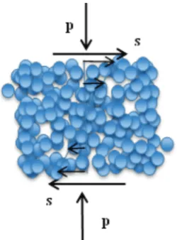
Here, we focus on continuous, steady, homogeneous shearing of a dense aggregate of identical spheres over a range of solid volume fraction,

φ

, above 0.49. We first consider theories that are appropriate in limits on either side of, but distant from, the critical volume fraction φ_c at which chains of spheres first span the flow.

Fig. 1: Steady, homogeneous shearing maintained by shear stress s and pressure p.

,

>

c

φ φ

we treat deformable spheres that interact through a constantly changing network of longer lasting contacts with multiple neighbors [25]. Finally, we join the two extremes over the entire range of dense volume fractions by incorporating contact deformation in the collisional regime and impulsive momentum transfer in the deformational regime [26].

We treat spheres with a diameter,σ, mass, m, Young’s modulus, E, Poisson’s ratio, ν, _friction

coefficient:μ, Normal restitution, e, and tangential restitution, β. _{The aggregate has a number density}

(

3

)

/ / 6 , =

n

φ πσ

mass density

ρ

=mn=

ρ φ

_p , where

p

ρ is the mass density of the material of the spheres, and is sheared at a rate u′.

2 Simple kinetic theory

The simplest kinetic theory [24] assumes instantaneous binary collisions, between a typical pair of frictionless, rigid spheres, with an impulse J exerted by sphere 2 upon sphere 1, and the change in velocities of the two spheres in a collision given by

′

c₁=c₁+J/ m and c′₂≡ ′c₂−J/ m (1)

where the prime denotes values after the collision. The component of the relative velocity c′₁₂≡ ′c₁− ′c₂, along the unit vector k directed from the center of sphere 1 to that of 2 is related to that before the collision by a coefficient of restitution e, with 0≤ <e 1:

(

)

12′ ⋅ = −e 12 ⋅ .

c k c k (2)

Then, the impulse may be determined as

12

1

m(1 e)( ) . 2

= + ⋅

J k c k (3)

The impulse figures in the calculation of the shear stress and pressure. The kinetic energy of the pair,

(

2 2

)

1 2 1

E m c c , 2

≡ + (4)

experiences the change

(

2

)

(

)

2 12 1

E E E m 1 e k c . 4

′

Δ ≡ − = − − ⋅ (5)

The change in kinetic energy is important when calculating the rate of collisional dissipation.

Averages over the exchanges of momentum and energy in collisions are carried out by integrating over a complete pair particle distribution that governs the likelihood of collisions between pairs of spheres. In the simplest dense theory, the positions and velocities of

colliding pairs are assumed to be completely uncorrelated - the assumption of Molecular Chaos - and the distribution is assumed to be expressed as the product of single particle velocity distributions and a correction to the collision frequency that incorporates the distance between edges, rather than centers.

The single particle velocity distribution is

(

)

2 (1)

3/ 2

( , ) exp ,

2 2

⎛ ⎞

= _⎜− _⎟

⎝ ⎠

c r n C

f

T T

π

(6)

where the velocity fluctuation

C r

( )

≡ −

c u r

( )

is given in

terms of the local average velocity _u(r), 2

,

≡ ⋅

C C

C

at

the point of contact r and the measure 2 / 3 ≡

T C of

the strength of the velocity fluctuations is often referred to as the granular temperature. The frequency correction is given in terms of the volume fraction dependence of the radial distribution function for a contacting pair in a dense aggregate [8]:

0

0.85

( ) .

0.64

g

φ

φ

=

− (7)

With these, the averages are carried out using the distribution function

(1) (1)

0( )r ( ,c r1 − k/ 2) ( ,c r2 + k/ 2),

g f

σ

f

σ

(8)

in which care is taken to distinguish between the locations of the enters of the colliding pairs and, in the simplest theory, spatial gradients of the average fields enter the theory through series expansions of these about the point of contact.

Integration yields expressions for the pressure

2(1

)

;

p

=

+

e GT

ρ

(9)

where

G

≡

ν

g

₀

,

the shear stress

1/ 2 /2

4(1 )

; 5

e

s

ρ σ

G T u

π

+ _′

= (10)

and the rate of collisional dissipation

2 3/ 2 1/ 2

12 1

. e

G T

γ

ρ

σ

π

−

= (11)

The last of these may be written as

γ =n 1

( )

−e2 1 2mT

24 π1/2

GT1/2

σ , (12)

frequency is the average time of flight,

τ

_f, between collisions:

1/ 2

1/ 2. 24 =

f

GT

π

σ

τ

(13)

In a steady, homogeneous shearing flow, the granular temperature is determined through the energy balance:

0.

′− =

su

γ

(14)

When the expressions for shear stress and the rate of dissipation are employed in this, it may be solved for T:

( )

(

)

2

2 2

. 15 1

′ =

− u T

e

σ

(15)

Then, the shear stress and the pressure can be expressed in terms of the shear rate:

( )

(

)

2 1/ 2

1/ 2 1/ 2

2 4(1 ) 2

15

5 ₁

u e

s G

e

σ

ρ

π

′ + ⎛ ⎞

= _{⎜ ⎟}

⎝ ⎠ ₋ (16)

and

( )

2 2 4(1 )

. 15 (1 )

′ +

=

− u e

p G

e

σ

ρ

(17)

We note for later comparison that the ratio s/p is independent of φ in the simplest theory.

3 Simple deformation theory

Pairs of spheres interact through contact forces that have normal and tangential components, P and T, parallel and perpendicular to their line of centers. In the simplest linear theory these are, respectively, proportional to the normal and tangential displacements δ and s of the contact. The normal force exerted by sphere 2 on sphere 1 is

, 4 =

P

π σδ

E (18)

while the tangential force is

, if 4

, otherwise.

⎧ _<

⎪ = ⎨ ⎪⎩

T

T E s P

P

π σ

μ

μ

(19)

The distribution of the magnitudes of the contact forces is roughly exponential [27]; so, for example,

1

( )= exp⎛_⎜− ⎞_⎟, ⎝ ⎠

P f P

P P (20)

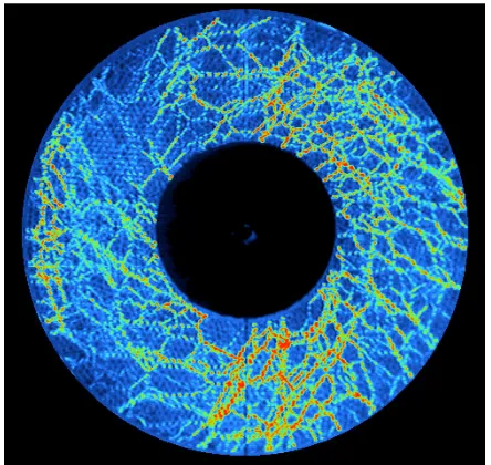
where Pis the average normal force. Discrete numerical simulations and physical experiments on photo-elastic disks indicate both the anisotropy and inhomogeneity of the distribution of contact forces in a sheared aggregate.

Fig. 2: Shearing of a planar aggregate of circular photo-elastic disks in the Behringer laboratory at Duke University,

http://behringer.phy.duke.edu/

The orientational distribution of contacts is described by a function A(k) of orientation k defined so that

A

( )

k

d

Ω

is the average number of contacts per particle within an element dΩof solid angle centered at k [25]. The average total number of contacts per particle Z is called the coordination number and is given in terms of A(k) by

( ) .

Ω

=

_∫∫

k Ω

Z A d (21)

When the contact distribution is isotropic,

( ) . 4 =

k Z

A

π

(22)

Anisotropic distributions of contacts are often described using a contact fabric tensor,a:

(

)

( ) 1

4 ij i j

Z

A a k k

π

= +

k (23)

with

a

ii

=

0.

Then,

15 1 1

( ) .

2 Ω 3

⎛ ⎞

= _⎜ − _⎟ Ω

⎝ ⎠

∫∫

ij i j ij

a A k k d

Z k

δ

(24)

( )

k

Ω

F k N

(

⋅ ΔΣ

)

,

nA

d

σ

(25)

for k N >⋅ 0. Similarly, for k N <⋅ 0. Taking half the

sum and integrating over all orientations k gives

( )

2

Ω

=

_∫∫

k

Ω

ij

n

i j

t

σ

A

F k d

(26)

For example, for an isotropic contact distribution, an average volume strain, Δ, positive in compression, and the contact displacement assumed to be given by the average strain, δ = σΔ/ 3, [25] thepressure is

1 . 12

= Δ

p Z E

φ

(27)

In applying this result to continued shearing beyond the critical volume fraction, it’s natural to relate the average volume strain to the excess of the volume fraction above the critical:

(

)

1

. 12

= − c

p Z E

_{φ φ φ}

(28)

Numerical simulations of very slow, continuous, homogeneous shearing [29] indicate that the stress is given by

.

=−+

ij ij ij

t

p

_δ

cpa

(29)

Because only axy is nonzero,

,

xy

s t

≡

=

η

p

(30)

With

(

)

1

, 12

= − c

p Z E

φ φ φ

(31)

and η yet to be determined.

4 Corrections to simple kinetic theory

In order to make realistic, quantitative predictions for dense, dissipative, shearing flows the simple kinetic theory whose derivation was outlined above has to be modified in a number of ways.

First, a more realistic complete pair distribution function must be derived and employed. This has been done for elastic spheres [30]. The resulting modification to the theory for steady, homogeneous shearing outlined above for dissipative spheres [2] requires that in the shear stress (10), the factor 1+e be replaced by the scalar factor J:

(

)

2

2 2

2 (1 ) (3 1)

1 .

96 24(1 ) 20 1

+ −

≡ + +

− − − −

e e

J e

e e

π

₍₃₂₎

Second, we must take into account the rotational degrees of freedom, and the additional loss of translational fluctuation energy to sliding, tangential restitution, and rotational fluctuation energy. This can be done by employing an effective normal coefficient of translation restitution, ε, that is derived using the balance of rotational fluctuation energy to determine the partition between rotational and translation energy in a steady, homogeneous flow. [31,32] The effective coefficient of restitution is simply expressed in terms of the coefficients of sliding friction and tangential restitution in two limits: when all contacts slide in a collision and

μ is about 0. 1,

2 9

, 2 2 = − +e

π

ε

μ

μ

(33)

and when all contacts come to rest at some time during a collision and μ is about 1,

2

2 2 1 1 5(1 )

4 4 1 .

7 7 9 5

⎡ ⎤

+ ⎛ + ⎞ +

= − + _{⎜ ⎟ ⎢}+ _⎥

−

⎝ ⎠ ⎣ ⎦

e β β β

ε

β (34)

Third, we must include the dependence seen in discrete numerical simulations of the critical volume fraction on friction. To do this, in g0 of Eq. (7), we

replace

0.64 by ( ),

φ μ

c where the dependence of φc on μ

is taken from the simulations [20].

Fig. 3: The stress ratio versus volume fraction in discrete numerical simulations, for frictionless particles, when e = 0.7: event driven simulations (hollow circles [10]); soft particle simulations (filled circles [33]). The solid and dashed lines are the predictions of simple and extended kinetic theory.

Finally, we must incorporate the influence of velocity correlations that occur above φ=0.49. At greater

which predictions and measurements of the ratio of shear stress to pressure versus volume fraction are shown for several typical systems.

A simple means of doing this is to introduce the cluster size in place of the particle diameter in the rate of collisional dissipation [12-14]

(

2

)

3/ 2 1/ 2

12

1 .

= G − T

L

ρ

γ

ε

π

(35)

The size of the cluster is determined by a balance between the orienting influence of the flow and the randomizing influence of the collisions:

1/ 2 ( ) ′, =

L u

F T

σ

φ

σ

(36)

where the

F

( )

φ

is proportional to

(

0.64−φ

)

−1[19]. That is, it is singular at random close-packing, not at the critical volume fraction. Then,

(

)

1/3 2

1/ 2 1 4

, 2

5

⎡ − ⎤

⎢ ⎥

=

⎢ ⎥

⎣ ⎦

s J

p JF

ε

π

(37)

where, in contrast to the ratio given by Eq. (16) and (17), there is a dependence on the volume fraction This relation is one of those plotted in Fig. 3, where it is referred to as that of the extended kinetic theory..

5 Deformation in collisions and

collisions in deformation

We next incorporate the deformation of the contacts during a collision into the collisional theory. [21] This provides a way to regularize the singularity in the collisional constitutive relations that without deformation occurs at the critical volume fraction.

When the deformation of a contact is linear, the duration, τc, of a contact is

1/ 2 , 5

⎛ ⎞ = ⎜ ⎟ ⎝ ⎠

p c

E

ρ

σ

τ

(38)

while we have seen that the time between collisions is

1/ 2

1/ 2. 24 =

f

GT

π

σ

τ

(39)

Consequently, if we take into account the duration of a collision, the time between collisions increases from τf to

τf +τf. In this case,

1/ 2 1/ 2 2 (1 ) (1 )

12

= + = +

f T

p ρ ε GT ρ ε π σ

τ (40)

becomes

1/ 2 1/ 2

(1 ) .

12 = +

+

f c

T

p _{ρ ε} π σ

τ τ (41)

Similarly,

2

15 ′

=

+

f c

J

s ρ σ u

τ τ (42)

and

(

2

)

1

1 .

2 f c

T L

σ

γ

ρ

ε

τ

τ

= −

+ (43)

With the incorporation of deformation into the collisions, the collisional stresses and the rate of dissipation are no longer singular at

φ φ

=

c

.

Fig, 4: Stress fluctuations below and above φc measured during

shearing in the circular annulus in the Behringer laboratory, http://behringer.phy.duke.edu/.

The need to incorporate dynamics in the range of volume fraction above the critical can be seen in the results of experiments carried out on photo-elastic disks. Here, a dramatic difference in the strength of the fluctuations in stress is seen in Fig. 4 below and above an area fraction that we identify with the critical. Consequently, for

φ φ

≥

c

,

there is still a collis-ional component of the exchange of momentum associated with the energy released by the breaking of chains. We assume that the frequency of these collisions is inversely proportional to the duration of a contact and evaluate the momentum transfer at the critical volume fraction.

(

)

1/ 2 1/ 2

(1 ) .

12 8

p c c

c T

p

ρ φ

ε

π σ

π

E

φ φ

τ

= + + − (44)

We treat the shear stress in a similar way, taking into account the relation (30) between the shear stress and pressure when deformations alone occur:

(

)

2

. 15 p c c 8 c

J

s

ρ φ

σ

u

η

π

E

φ φ

τ

′

= + − (45)

In this regime, we assume that the anisotropy of the collisions is the same as that of the deformation and take

η to be the ratio of the collisional shear stress to the collisional pressure at φc:

1/ 2 1/ 2

4 1

. (1 ) 5

J u

e T

σ

η

π

′ =

+ (46)

Finally, in order to enable the determination of the strength of the velocity fluctuations at volume fractions greater than the critical, we adopt similar assumptions for the frequency of collision and the volume fraction in the rate of collisional dissipation:

(

2

)

1

1 .

2 p c c

T L

σ

γ

ρ φ

ε

τ

= − (47)

Then, in simple shearing flows, both below and above the critical volume fraction, T may be obtained as a solution to the energy balance (14). In this energy balance, the elastic part of the shear stress above the critical volume fraction is assumed to be recoverable and not to contribute to the rate of working.

6 Results

With T determined on either side of the critical volume fraction, the stress may be calculated and compared to the results of discrete numerical simulations [20,33,34]. The comparison for the pressure and shear stress,

normalized by

ρ σ

p

( )

u′ 2, are shown in Figs. 5 and 6,

respectively, for a wide range of contact stiffness,

(

/ 4

)

E ,

κ π

≡

σ

made dimensionless by

ρ σ

p 3

( )

u′2. The

predictions are, in general, good and provide an indication that at least some of the numerous assumptions made to obtain them have a basis in the physics.

A more stringent test results from plotting the ratio of the shear stress to the pressure. In this case, because he stiffness is assumed to enter into both quantities in the same way, the ratio is independent of stiffness. In contrast. the measured data is sensitive to the stiffness, especially for the more compliant spheres. The agreement for the stiffer spheres is relatively good.

Fig 5: Predictions of the normalized pressure versus volume fraction for e = 0.7, μ = 0.5, values of the dimensionless contact stiffness ranging from 10 to 1011 (dashed curves) and data from the discrete numerical simulations [20,33,34].

Fig 6: Predictions of the normalized shear stress versus volume fraction for e = 0.7, μ = 0.5, values of the dimensionless contact stiffness ranging from 10 to 107 (dashed curves) and data from the discrete numerical simulations [20,33,34].

0.5 0.55 0.6 0.6

φ

0.3 0.35 0.4 0.45 0.5 0.55 0.6 0.65 0.7

s/p

7 Conclusions

We have outlined the derivation of a theory for steady, homogeneous shearing flows of dense aggregates of deformable, dissipative spheres. The incorporation of contact deformation in the collisional regime and impulsive momentum transfer in the deformational regime permits a smooth transition through the critical volume fraction and relatively good descriptions of the stresses on either side of it. The predictions compare well over the range of volume fraction before and after the hard sphere singularity and over nine orders of magnitude of the contact stiffness. The model requires no parameters other than the contact stiffness, and the coefficients of restitution and sliding friction of the spheres.

References

1. J.T. Jenkins, S.B. Savage, J. Fluid Mech. 130, 187–202 (1983)

2. V. Garzo, J.W. Dufty, Phys. Rev. E 59, 5895–5911 (1999)

3. I. Goldhirsch, Annu. Rev. Fluid Mech. 35, 267–293 (2003)

4. E. Azanza, F. Chevoir, P. Moucheront, J. Fluid Mech. 400, 199–227 (1999)

5. Y. Forterre, O. Pouliquen, Phys. Rev. Lett. 86, 5886 (2001)

6. H. Xu, M. Louge, A. Reeves, Continuum Mech. Thermodyn. 15, 321–349 (2003)

7. B.J. Alder, T.E. Wainright, J. Chem. Phys. 27, 1209 (1957)

8. S. Torquato, Phys. Rev. E 51, 3170–3182 (1995)

9. N. Mitarai, H. Nakanishi, Phys. Rev. Lett. 94, 128001 (2005)

10. N. Mitarai, H. Nakanishi, Phys. Rev. E 75, 031305 (2007) 11. V. Kumaran, J. Fluid Mech, 632, 145–198 (2009) 12. J.T. Jenkins, Phys. Fluids 18, 103307 (2006) 13. J.T. Jenkins, Granular Matter 10, 47–52 (2007)

14. J.T. Jenkins, D. Berzi, Granular Matter 12, 151–158 (2010)

15. D. Berzi, Acta Mech. 225, 2191–2198 (2014) 16. D. Berzi, J.T. Jenkins, Phys. Fluids 23, 013303 (2011) 17. J.T. Jenkins, D. Berzi, Granular Matter 14, 79–84 (2012) 18. D. Vescovi, D. Berzi, P. Richard, N. Brodu, Phys. Fluids

26, 053305 (2014)

19. D. Berzi, D. Vescovi, Phys. Fluids 27, 013302 (2015) 20. S. Chialvo, J. Sun, S. Sundaresan, Phys. Rev. E 85, 021305 (2012)

21. H. Hwang, K. Hutter, Continuum Mech. Thermodyn. 7, 357–384 (1995)

22. P. Johnson, P. Nott, R. Jackson, J. Fluid Mech. 210, 501–535 (1990)

23. D. Berzi, C. di Prisco, D. Vescovi, Phys. Rev. E 84, 6 (2011)

24. J.T. Jenkins, S.B. Savage, J. Fluid Mech. 130, 187- 202, (1983)

25. J.T. Jenkins, O.D.L. Strack, Mech. Mater. 16, 25–33 (1993)

26. D. Berzi, J.T. Jenkins, Soft Matter 11, 4799-4808 188303 (2015)

27. C. Thornton, KONA 15, 81-89 (1997)

28. J.T. Jenkins, in Modern Theory of Anisotropy Elasticity and its Applications, 368-377, SIAM (1990) 29. J. Sun, S. Sundaresan, J. Fluid Mech. 682, 590–616 (2011)

30. S. Chapman, T.G. Cowling, The Mathematical Theory of Non-Uniform Gases, Cambridge University Press,

3rd

Ed. (1970)

31. J.T. Jenkins, C. Zhang, Phys. Fluids 14, 1228 (2002) 32. M. Larcher, J.T. Jenkins, Phys. Fluids 25, 113301 (2013) 33. S. Chialvo, S. Sundaresan, Phys. Fluids 25, 070603 (2013)