INHERITANCE OF QUANTITATIVE CHARACTERS IN RICE. I. ESTIMATION OF THE NUMBER OF EFFECTIVE FACTOR PAIRS CONTROLLING PLANT HEIGHT

(1)

INHERITANCE OF QUANTITATIVE CHARACTERS IN RICE.

I. ESTIMATION OF THE NUMBER OF EFFECTIVE FACTOR PAIRS CONTROLLING PLANT HEIGHT

ALY H. MOHAMED AND AMIN S. HANNA

Department of Genetics, Faculty of Agriculture, Alexandria Uniuersity, Alexandria, Egypt, U.A.R.

Received August 1, 1963

is a well known fact that the basis of inheritance of quantitative characters ';epends on genes subject to the same laws of transmission and having the same general properties as the genes whose transmission and properties are displayed by qualitative characters. We may expect them to show variation in dominance, gene interaction, linkage, etc. In that way, quantitative inheritance is an exten- sion of the general Mendelisms. However, when dealing with quantitative characters we are dealing with quantity and continuous variation. Thus, the distinction between genes concerned with qualitative characters and those concerned with metric ones lies in the magnitude of their effects relative to other sources of variation. Variations in environment are likely to add to variation in the characters, bringing about a lower correlation between genetic make up and degree of expression of the characters. In this system the effects of most genes are integral parts (WRIGHT 1934).

In such studies it is necessary to separate the environmental variance from the genetic one. Furthermore, statistical techniques must be used rather than simply counting the number of individuals belonging to a few easily distinguishable classes.

Numerous methods of analysis for determining the number of effective factor pairs controlling the expression of a quantitative character as well as determining factor action have been developed by many workers. These methods of analysis must be based on assumptions to set up a genetic model that will agree well with the observed data. Due to the fact that some of these assumptions seem to be highly improbable (CASTLE 1921), many geneticists felt that any method of analysis that falls short of the actual isolation of the effective factors involved means little. Therefore various methods have been suggested by POWERS (1939, 1942, 1950, 1951), POWERS, LOCKE and GARRETT (1950), WTHER (1949a, 1949b), MATHER and VINES (1952), LEONARD, MANN and

POWERS

(1957), and many others.

The effective factor has been described by MATHER (1949a) as the smallest unit of hereditary material that is capable of being recognized by the methods of biometrical genetics. It may be a group of closely linked genes, o r at the lower limit, a single gene.

(2)

82 A. H. M O H A M E D A N D A. S. H A N N A

The present studies were undertaken to determine the mode of inheritance of plant height in the cultivated rice plant, Oriza sativa L.

M E T H O D S A N D M A T E R I A L S

Two commercial rice varieties, obtained from the Plant Breeding Section, Ministry of Agri-

culture, Egypt, U.A.R., were used in this study. These two varieties were Sabini (P,) and

Pakistan-7 (P,). The Sabini variety is local to Egypt and its origin is unknown. This denomina-

tion was given to this variety since the panicles are produced in about 70 days from planting. Economically it is considered to be of a low grade and therefore it is usually grown as a Nile crop (short season) in the Fayoum province. On the other hand, the Pakistan-7 variety was intro-

duced by the Egyptian Ministry of Agriculture (date of introduction is uncertain). I t is one of

the main varieties that entered into the program for improving the cultivated rice in Egypt.

The crosses between the two varieties were made in the summer of 1958. The F, seeds as well

as the parents were grown i n 1959 in plots 1 meter x 3 meters. The parent, F, and F, seeds were

sown in the same way in 1960. Plots of the parental varieties were interspersed between the F,

plots. In 1961, the design was a modified randomized complete block consisting of six blocks.

Each block contained four plots of F,, one plot of PI, P, and F, and 70 plots of F,. Each plot

contained eight plants. In order to minimize the effects of plant competition, seeds of the F,, F,,

F, and the parents were spaceplanted at one-foot intervals in rows spaced one foot apart.

.

The plants were allowed to grow to maturity before the character was recorded. Plant height was determined by measuring the tallest culm of each plant from the soil level to the top of the

panicle to represent the main stem (HECTOR 1936).

I n testing for the number of effective factor pairs controlling plant height and the type of factor interaction, two commonly used methods were applied. The first one was that discussed by

POWERS (1942, 1950, 1951), POWERS, LGCKE and GARRETT (1950), and LEONARD et al. (1957).

The second method was that suggested by MATHER (1949a, 1949b) and MATHEB and VINES

(1952) for utilizing the F, generation.

E X P E R I M E N T A L R E S U L T S

1. The partitioning method utilizing the F , data: The first procedure in study-

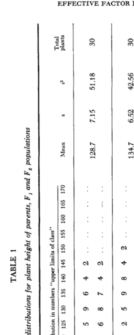
ing any continuous character is to determine which scale the variability will follow. The obtained arithmetic means for plant height and the number of plants for the different populations are given in Table 1. If the data were following the arithmetic scale, then the F, mean should equal, within the limits of sampling error, the mid-point of the two parents (1 16.8 cm)

,

but such was not the case. On the other hand, if the genetic variability were following the logarithmic scale, then the F, mean would be 116.2 cm. This also was not the case. Thus it could be seen that gene effects do not follow either of the two scales.

(3)

TABLE 1 Obtained frequency distributions for plant height of parents, F, and F, populations Frequency distribution in numbers “upper limits of class” Total Population 95 100 105 110 115 120 125 130 135 140 145 150 155 160 165 170 Mean S S= plants

8

%

m

Sabini Obtained ... Theoretical ... (Pl) .. 459642 ... .. 368742 ... LJ ..

?I 4 M

128.7 7.15 51.18 30 .. h Obtained ... Theoretical ... Fl .. 25 9842 ... .. 2 513 4 5 1 ...

4 0 F w >

134.7 6.52 42.56 30 Y Obtained 2 6 12 17 31 30 54 51 62 49 38 14 12 6 1 2

z

E

Theoretical 3 5 10 22 24 42 52 55 54 46 33 21 12 6 2 1 M 128.3 13.5 184.15 387 0

F2 Pakistan-7

Obtained 3 4 9 6 5 3 ... (P,) Theoretical 3 5 5 10 5 2 ... .. .. 105.0 7.28 53.02 30

(4)

TABLE

2

Frequency

distributions

of

obtained

data

of

parents,

F,

and

F,

populations

expressed

as

percentages

Upper

class

limit

Total

Population

95

100

105

110

115

120

125

130

135

1W

145

150

155

160

165

170

plants

Sabini

(P,)

13.3

16.7

30.0

20.0

13.3

6.7

30

Fl

6.7

16.7

43.3

13.3

16.7

3.3

30

F2

0.8

1.3

2.6

5.7

6.2

10.9

13.4

14.2

13.9

11.6

8.5

5.4

3.1

1.6

0.5

0.3

387

Pakistan-7

(P,)

10.0

16.7

33.3

16.7

6.6

..

(5)

EFFECTIVE FACTOR PAIRS I N RICE 85

bility in making an analysis of such data. This could be accomplished by working out the individual genotypes of the different populations.

Since the arithmetic scale was used in recording the data, it would be necessary to ascertain first whether the variability followed the normal probability integral (LEONARD et al. 1957). For testing for normality, the observed frequency distributions were compared with the calculated (Table 1) by means of a chi-square test for goodness of fit. Some adjacent classes, at the tails in Table 1, were grouped together to provide the theoretical frequency of at least ten individuals in each of the tail classes. The chi-square test could not be applied for the two parents and the F, population, since the number of plants in each was small, and after com- bining the adjacent classes to provide at least ten individuals in each class of the theoretical frequency, only two degrees of freedom would be left. These two degrees of freedom would not fulfill the three restrictions mentioned by LEONARD

et al. (1957). For the F, population, chi-square was 11.82, with P between .20

and .lo, indicating that the obtained distribution agreed well with the theoretical normal one.

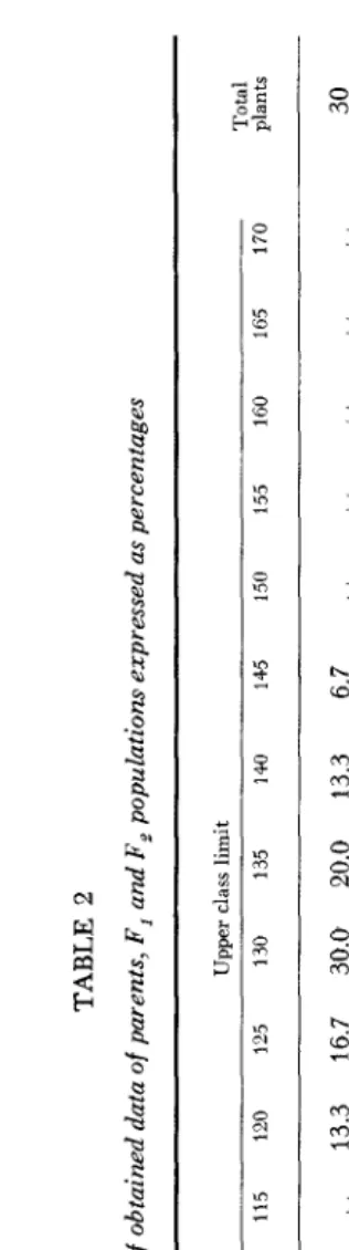
Number of eflective factor pairs differentiating parents: I t could be seen from

Table 2 that the F, frequency distribution, expressed in percentages, was uni- modal. The mode occurred in the 130-class with a value of 14.2 percent. It could also be seen that this mode corresponded to that of Sabini (P,). The mode in Pakistan-7 (P,) fell in the 110-class with a value of 33.3 percent. When all percentage values in the 120-class and the lower classes were added in the F, distribution, a value of 27.5 percent was obtained. When the 125 and higher classes were added, a value of 72.2 percent was obtained. This indicated that one effective factor pair conditioned plant height in the F, population.

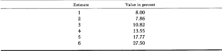
However, the fact that the mode for the 120 and higher classes failed to cor- respond with the mode of P, indicated that at least one other effective factor pair was involved. Therefore, the simplest possible hypothesis was that two effective factor pairs differentiated the two parents with respect to plant height. This indi- cation was arrived at by using the formula F,/P, (POWERS 1955). It can be seen from Table 3 that the first three estimates appeared to fluctuate around a value of 6.25, indicating that the parents were differentiated by two effective factor pairs. These three classes represent the double recessive genotype. According to LEON-

ARD et al. (1957) the rise in the other estimates would indicate that individuals

TABLE 3

Calculated values used for the estimation of effective factor pairs involved

Estimate Value in percent

1 8.00

2 7.86

3 10.82

4 13.55

5 17.77

(6)

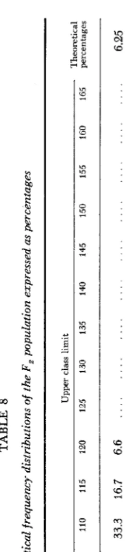
TABLE 4 Partitioning the frequency distribution of the F, population on the basis of the frequency distributions of the two parents Upper class limit

Theoretical percentage

(7)

with genotypes other than that of the double recessive occurred in the 110 and other classes. Accordingly, the genotype of Sabini (PI) was symbolized as AABB

and of the Pakistan-7 (Pz) as aabb.

When plants of the AaBb genotype fall in the same classes of the frequency distribution as plants of the AABB genotype, it follows that plants of the AABb

and AaBB genotypes also will fall in the same classes. Consequently, the expected

percentage of the F, population that will fall in the same classes as Sabini (PI)

would be 56.25. This corresponds to the ratio 1 : 2: 2: 4 of the double dominant class of a dihybrid.

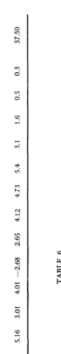
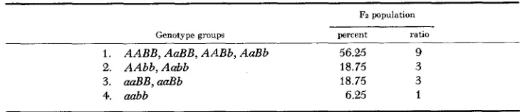
Following this, the F, frequency distribution was partitioned on the basis of the frequency distribution of the two parental lines (Table 4 ) . The theoretical percentages listed in the last column of Table 4, together with the obtained frequency distributions of PI and Pz were used to estimate the theoretical frequency distributions of plants having the genotypes AABB, AaBB, AABb and AaBb, and those with the genotype aabb, respectively. The values in the second and the third rows of Table 4 are the theoretical frequency distributions of the plants with the designated genotypes. After subtracting these values from the obtained percentages of the F, population, the frequency distribution of the balance of the plants with the genotypes AAbb, Aabb, aaBB, and aaBb was obtained.

The fact that the frequency distribution (Table 4, last row) exhibited two peaks, one at 5.16 (1 15-class) and the other at 5.4 (150-class), indicated that Aa

and Bb gene pairs had effects of different magnitude. This also indicated complete genic dominance. The complete genetic hypothesis expressed in percentages and ratios is given in Table 5. To arrive at the means and standard error for the genotypes of groups 2 and 3, the method described by LEONARD et al. (1957) was used. Since the frequency distributions of the two parents followed the normal curve, it was possible to estimate the theoretical frequency distribution of the plants with the genotypes AAbb

4-

Aabb and aaBB 4- aaBb (Table 6 ) . Th' is was computed from the balance given in Table 4. The estimated total variances from the different genotype groups are given in Table 7. It can be seen from this Table that the theoretical standard errors of the means of the genotypes supported the assumption that the F, population was made up of a composite of genotypes, each of which fluctuated about its own mean.

On the other hand, the four theoretical frequency distributions of the nine F,

genotypes (Table 8) were calculated by the method discussed by POWERS et al.

TABLE 5

Complete genetic hypothesis expressed as percentages and ratios

~~~ ~

Fz population

Genotype groups percent ratio

1. AABB, AaBB, AABb, AaBb 56.25 9

2. AAbb,Aabb 18.75 3

3 . aaBB,aaBb 18.75 3

(8)

88 A. H. M O H A M E D AhTD A. S. H A N N A

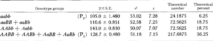
TABLE 7

Statistical constants and theoretical ualues for estimation of theoretical frequency distributions

Theoretical Theoretical

Genotype groups Xi-S E SZ S number percent _--

aabb (P,) 105.0 -C 1.480 53.02 7.28 24.1875 6.25

d B

+

aaBb 110.6 t 0.851 52.58 7.25 72.5625 18.75

A A b b

+

Aabb 143.0 & 0.830 50.07 7.07 72.5625 18.75

AABB

+

A A B b

+

AaBB

+

AaBb (P,) 128.7 -C 0.480 51.18 7.15 217.6875 56.25

( 1950). The

x2

test for homogeneity between the obtained and calculated F, frequency distributions gave a value of 14.06, with P between .10 and .05 (Table 9). The degrees of freedom in this test were 8 instead of 10. This is due to the fact that two degrees of freedom were lost in the calculations of the theoretical means of the frequency distributions of the A A b b

+

Aabb and aaBB

+

aaBb genotypes

(FISHER 1950). The obtained P value indicated a good fit and supported the

hypothesis that the two parents were differentiated by two effective factor pairs with respect to plant height.

Effective magnitude and interaction: The magnitude of the effective factor

effects as well as interaction was determined through the comparisons between the means and standard errors (LEONARD et at. 1957).

(a) Effect of (A-a) factor pair:

First estimate: 143.02 f 0.83 - 105.00 f 1.48 = 38.02 t 1.69

Second estimate: 128.70 k 0.48 - 110.60 i. 0.851 = 18.10 i: 0.977

First estimate: 110.60 f 0.851 - 105.00 i 1.48 = 5.60 I. 1.707

Second estimate: 128.70 -C 0.48 - 143.02 f 0.83 = -14.32 I 0.958.

It is obvious from these estimates that ( A - a ) factor pair had approximately seven times the effect on plant height of the (B -b ) factor pair.

(b) Effect of (B-b) factor pair:

Testing for effective factor interaction, the estimates were: (a) Effectiue factor pair (A-a):

(b) Effectiue factor pair (B-b) :

38.02 +- 1.69 - 18.1 t 0.977 = 19.92 t 1.95

5.60 f 1.707 - (-14.32) t 0.958 = 19.92 t 1.95

Thus, it can be seen that the two values were identical.

2. T h e partitioning method utilizing the F , duta: In this part of the analysis, all

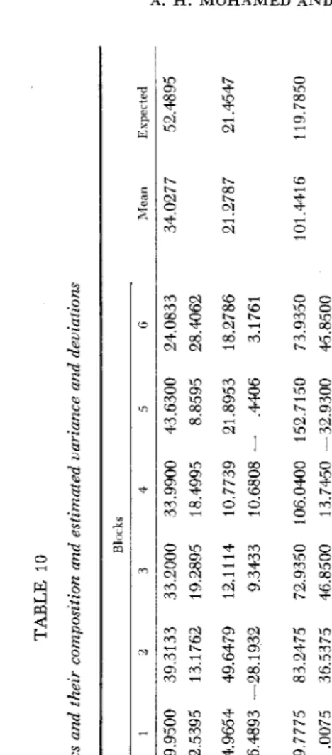
plots of P,, P,, F,, F, and F, populations were of the same size, i.e., eight plants per plot. The nonheritable components of variation in the F, and F, generations could, however, be assumed to be the same. An estimate of this component was obtained from the variances of the nonsegregating generations. A reasonable estimate of the nonheritable component ( E , ) in F, and F, generations was taken as the mean of the three variances of the two parents and the F, i n each block. For example, for Block 1 this was 1/3 (25.64

+

41.71

+

22.50)= 29.95 as entered in Table 10.

(9)

(10)

TABLE 10 The different statistics and their composition and estimated variance and deviations Blocks Stvtistir Coniposition 1 2 3 4 5 G Mean Expected El E, E2 E2

Deviation Deviation

u2 F

%D

+

?4H

+

E, '/zD

4-

~BH f E, Deviation U2 3 Deviation

-

U2

3 %D

+

%H

+

El Deviation F /F cov 2 3

'/zDi-%H Deviation

(11)

E F F E C T I V E FACTOR P A I R S I N R I C E 91 every block, E,, the between group nonheritable variance cannot be estimated directly. However, the equation U?=

E,

4-

u2 could be used. I n this equation U’

is the sampling variance and it is equal to

i/e

(%*-

E , ) .

FZ S

The F2 variance ( u 2 )

,

variance of F, means (U?-), covariance of F, means and

F, plant values (cov

F,/F,)

and mean variance of F3’s

(3

) are set out together with the estimates of the two nonheritable components in Table 10. Since six estimates of each statistic were available from the six blocks, six values appeared in each line of Table 10. The average of the estimates was used in partitioning the variation. The differences between estimates then are available for finding the standard errors of the estimates of the various components of variation (MATHER

1949a, 1949b).

The estimated values of the four components of variation

D,

H , E , and E, could be arrived at by using the six basic formulae (MATHER 1949a) :

FZ Fa

F3

0 2

2 = %D+i/,H+E, = 101.4416

= l/,D+&H+E, = 4.5337

= % D + ? W + E l = 122.6929

cov

= % D f % H = 40.0277

= 34.0277

= 21.2787

By solving, the estimation for

D

was 27.3028 33.32, for H 214.5764 f 106.624,

for E , 52.4895 f 9.0742 and for

E2

21.4548 f 9.1252. Then by substituting these

estimated values for the composition of u2 for example, the expected value

48.51 72 was obtained. This and the other constants obtained by the same way are given in Table 10. The six values for any statistic obtained in each block deviated from the expected value. There are 36 such deviations had 32 degrees of freedom since four degrees have been sacrificed in estimating the four parameters

D,

H , E,, and E,.

Number of effective factor pairs differentiating parents: For estimating the

number of effective factor pairs, the mid-parent value was calculated. It was found to be 109.025. Beside the deviation of either parent, the value for 2 (d,)

should be obtained. This was found to be 10.905. Then if all the genes gave equal increments, )3 (d,) should equal Kd, where K equals the number of effective factor pairs (MATHER 1949a). In this case

D

= (d,) = Kd2. Thus, on obtaining these values the number of effective factor pairs could be arrived at from the formula

( K d ) 2 / K d 2 . This was found to be 4.35. Therefore, it could be concluded that the estimated number of effective factor pairs differentiating the two parents with respect to plant height was four.

- -

F2/F3

El

E2 - -

F3’

D I S C U S S I O N A N D C O N C L U S I O N

(12)

92 A. H. M O H A M E D A N D A. S. H A N N A

quency distribution of any segregating population into its component genetopes. Tests for the validity of the genetic hypothesis can be accomplished through comparisons between the obtained and theoretical means, frequency distributions and variances (POWERS et al. 1950).

The two parental lines, Sabini and Pakistan-7, were found to be differentiated by two effective factor pairs with respect to plant height by applying the partitioning method developed by LEONARD, MA", and POWERS (1957). The genetic constitution of Sabini and Pakistan-7 was designated as AABB and aa bb respectively. It was also found that the ( A d ) factor pair had approximately seven times as great an effect on plant height as the (B-b) factor pair. In applying this method, its limitations should be realized (POWERS 1963). When the number of the effective factor pairs differentiating the parents increases, the reliability of

POWERS' method decreases. Also, there should be a fairly high number of indi-

viduals for all the populations involved. The number of individuals in the PI, P,

and F, populations in this study was somewhat limited, which could, to a certain extent, reduce the validity of the conclusion reached. This was not intentional but was due to difficulties in rice cultivation. Also extensive genetic design is de- sirable as a basis for the final genetic conclusion. Such an adequate design in- cludes backcrosses and advanced generations (POWERS 1939, 1942, 1955, 1963). A different result, however, was obtained by using the partitioning method based on MATHER'S method (MATHER 1949a, 194913; MATHER and VINES 1952).

The number of effective factor pairs was estimated to be four. This finding is, however, an unreliable one since the estimates of H ,

D,

and E components of variance were themselves unreliable estimates. These values cannot be expected to give a reliable estimate of the number of effective factor pairs differentiating parents. This is particularly true since it has been found that the effective factors involved do not give equal increments. Also, in the presence of interaction, which has been revealed, not only are the relations

D

=

z

($) and H =

z

( P )

no longer strictly true, but also the magnitude of disturbance will vary between the different variances and covariances (MATHER 1949a). It should also be realized that the

F, and F, data by themselves can seldom be expected to give a very precise value of H .

The high standard errors attached to

D,

H , and E, and the values of the statistics expected on the basis of these estimates, do reflect the unreliability of these estimates. Thus, our estimate of the number of the effective factor pairs, estimated from F, data, will be rejected on this ground.

In any case, the findings with regard to the number of the effective factor pairs will not be conclusive unless further data are available in which marker genes are used. Association tests between the effective factor pairs and well defined qualitative genes should be carried out to reach a reliable conclusion.

SUMMARY

The rice variety Sabini was crossed to the variety Pakistan-7 and their F,, Fz,

(13)

LEONARD, MANN, and

POWERS

( 195 7), it was possible to estimate, from the

F2

generation, the number of effective factor pairs differentiating the two parents with respect to plant height. Also the results obtained by this method were compared with those obtained from the partitioning method suggested by MATHER

(1949a, 1949b) and MATHER and VINES (1952) for utilizing the F, data. The two parents were found to be differentiated by two effective factor pairs with respect to this character, by using POWERS’ method. However, the number of the effective factor pairs found by using MATHER’S method was estimated to be four. This last conclusion was found to be unreliable. The interaction between the two nonallelic factors found by POWERS’ method, was also determined. There was complete phenotypic and partial genic dominance for plant height and heterosis seemed to exist. The validity of the two methods was discussed with respect to the estimation of the number of effective factor pairs differentiating parents.

LITERATURE CITED

CASTLE, W. E., 1921 On a method of estimating the number of genetic factors concerned in

cases of blending inheritance. Science 54: 93-96.

FISHER, R. A., 1950 Statistical Methods for Research Workers. 11th edition. Oliver and Boyd, Edinburgh and London.

HECTOR, J. M., 1936 Introduction to the Botany of Field Crops. 2 volumes. Central News

Agency, Johannesburg, South Africa.

LEONARD, W. H., H. 0. MANN, and L. POWERS, 1957 Partitioning method of genetic analysis

applied to plant-height inheritance in barley. Colorado Agr. Exp. Sta. Tech. Bull. 60. 24 pp.

MATHER, K., 1949a Biometrical Genetics. Methuen, London. - 1949b The genetical

theory of continuous variation. Proc. 8th Intern. Congr. Genet. (Hereditas Suppl. Vol.): 376-401.

The inheritance of height and flowering time in a cross of Nicotiana rustica. Pp. 49-80. Quantitative Inheritance. His Majesty’s Stationery Ofice, London.

POWERS, L., 1939 Studies on the nature of the interactions of the genes differentiating quantita-

tive characters in a cross between Lycopersicon esculentum and L. pimpinellifolium. J.

Genet. 39: 139-190. - 1942 The nature of the series of environmental variances

and the estimation of the genetic variances and the geometric means in crosses involving

species of Lycopersicon. Genetics 27: 561-575. __ 1950 Gene analysis of weight per

locule in tomato hybrids. Botan. Gaz. 112: 163-174. - 1951 Gene analysis by the

partitioning method when interactions of genes are involved. Botan. Gaz. 113: 1-23.

-

1955 Components of variance method and partitioning method of genetic analysis applied

to weight per fruit of tomato hybrid and parental populations. U.S. Dept. Agr. Tech. Bull.

1131: - 1963 The partitioning method of genetic analysis and some aspects of its

application to plant breeding. Statistical Genetics and Plant Breeding. Natl. Acad. Sci.-Natl.

Res. Council Publ. 982: 280-318.

Partitioning method of genetic analysis

applied to quantitative characters of tomato crosses. U.S. Dept. Agr. Tech. Bull. 998. 56 pp.

Physiological and evolutionary theories of dominance. Am. Naturalist 48:

24-53.

MATHER, K., and A. VINES, 1952

POWERS, L., L. F. LOCKE, and J. C. GARRETT, 1950