RANK-ORDER SELECTION IS CAPABLE OF MAINTAINING ALL GENETIC POLYMORPHISMS

(1)

RANK-ORDER SELECTION IS CAPABLE

OF

MAINTAINING ALL GENETIC POLYMORPHISMS

CHRISTOPHER WILLS

Dept. of Biology, University of California at San Diego, La Jolla, California 92093

Manuscript received June 9, 1977 Revised copy received December 27, 1977

ABSTRACT

The fitness of organisms may be due chiefly to a fitness curve imposed on

their ranking in the population with respect to heterozygosity. If this is so,

then the number of polymorphisms that can be retained at a particular selective equilibrium increases as the square of the population size. All of the genetic variation that we currently observe and infer to exist can probably be maintained by selection in a papulation of about I O 5 individuals. Selection

acting i n this way is so strong that these polymorphisms can be expected to behave very differently from neutral ones.

I T

is generally agreed that selection based on strictly multiplicative fitnesses is inadequate to explain the amount of polymorphism observed in natural populations. In the multiplicative model, the fitness of an individual homozygous at

n loci can be represented by (1 - s)~, where s is the selection coefficient associated with homozygosity at each locus. As

LEWONTIN

and

HUBBY

(1966) pointed out, if s is sufficiently large that selection, rather than drift, has the predominant effect on allele frequencies at each locus, then the load quickly becomes so great as to threaten extinction of the population as the number of segregating loci becomes large. Indeed, this was one of the arguments employed by KIMURA (1968) to explain why he considered that the great majority of observed genetic polymorphisms must be selectively neutral.

Several alternative forms of selection have been proposed (SVED, REED and

BODMER 1967; KING 1967; MILKMAN 1967; TOBARI and KOJIMA 1967) in order to circumvent this problem. I wish in this paper to present some consequences of the selection model proposed by MILKMAN (1967)

,

following a suggestion of

MAYR (1959). A less quantitative version of this model, termed “soft selection,” was discussed by WALLACE (1968, 1975). This model, or a modification of it,

can provide for selection of all observed genetic variability.

I

will give an analytical model showing the numbers of polymorphisms that can be maintained with this type of selection, which I would like to term rank-order selection.

I will also discuss the magnitudes of the selection coefficients that can be expected to be associated with these polymorphisms, and show that rank-order selection permits them to be so large that the behavior of these polymorphisms can be

(2)

404 c . WILLS

expected to be very different from that of neutral polymorphisms. I n a later paper, I will deal with the effect of linkage disequilibrium on multigenic systems subject to rank-order selection.

RANK-ORDER SELECTION

Let me begin by formalizing the concepts that underlie MILKMAN’S (1967) type of selection. In his view, it is the relative ranking of organisms with respect to some variable that in conjunction with the environment determines their fitnesses. This immediately circumvents the difficulty inherent in the multiplicative model in which fitness is given by an absolute genotypic value, since fitness becomes relative rather than absolute. What is this underlying variable that determines the rank order of the organisms in the population? MILKMAN

(1973) termed it the organism’s “fitness potential,” since it is only indirectly translated into fitness; the final fitness value is determined by the relative ranking of the organism’s fitness potential among those of the rest of the population, and by the severity of the environment. The environment may impose a distribution of fitnesses on this ranking in such a way that certain organisms may not reproduce at all, even though they may be perfectly capable of doing so under less severe circumstances. This is a truncation, of the sort familiar to quantitative geneticists, and it may take many forms. Modifications of this simple model will be considered later in the paper.

It is worth noting that under the multiplicative model all organisms not homozygous for a lethal have a non-zero chance of reproduction. The range of fitnesses in a population subject to multiplicative selection is not great. For example,

if 1000 loci are segregating in such a population, and at each locus s1 = s4 = 0.001, then the mean fitness of the population is 0.999500 = 0.606, and 95% of the population will have fitnesses lying between 0.999532 = 0.587 and 0.999468 = 0.626.

A

truncation model immediately introduces the possibility of a fitness of zero, so that the range of fitnesses in the population can be enormously greater. Fur- ther, and this is an important difference. in the multiplicative model the effective size of the population is immediately affected by the distribution of genotypes and, therefore, (since the two are perfectly correlated on a log-linear scale) by the distribution of fitnesses. In a rank-order or other truncation model, the effective size is a function of the distribution of fitnesses, but not a direct function of

the distribution of genotypes in the population. Truncation permits large differences in fitness even if the effective population size remains large. Because of this divorcing of effective population size from the distribution of genotypes, it is possible under the rank-order model to impose approximately equal amounts of selection on a per organism basis in populations with very different ranges of fitness potential. This will occur if the distribution of fitnesses imposed on these different populations by the environment is approximately the same in each case.

(3)

RANK-ORDER SELECTION A N D P O L Y M O R P H I S M 405

in this property, but be much less fit if it is transported to a population in which most of the organisms have a higher fitness potential.

The fitness potential undoubtedly has many components. The one with which we will be concerned here, however, is that component which leads to the maintenance of polymorphisms by balancing selection. This paper deals with simple heterotic selection, but regardless of the mode of balancing selection at each locus-single-gene heterosis, marginal overdominance, geometric mean overdominance ( PELSENSTEIN 1976) or frequency-dependent selection-the upshot is that for polymorphisms to be maintained the heterozygote must have or must appear to have the highest average fitness. In actuality, the relative contribution to this component of fitness potential by different loci and by different genotypes at a locus must vary greatly, but I will use here

MILKMAN’S

original simplified model in which fitness potential is directly proportional to average heterozygosity. As will be developed later, I do not consider that small deviations from this simple model will have a large effect on the consequences for the maintenance of polymorphism.

There are several limitations associated with the rank-order model. I will mention two here and others at the end of the paper. The first is that only that component of fitness potential which leads to the maintenance of balanced polymorphisms will be considered in this discussion. Transient selected polymorphisms will also contribute to the fitness potential; there will, of course, be a large environmental component. and there will be a component of uncertain size contributed by genes exhibiting a very low genotype-environment interaction. These latter genes, chiefly lethals and severe subvitals, make up the mutational load and are not usually polymorphic in the accepted sense.

I

have pointed out elsewhere (WILLS 1973) that genes which are not of the mutational load type, but rather are of the sort that should be subject to rank-order selection, will tend to accumulate in natural populations if they arise at all, and that such genes are simply polymorphisms in which all the alleles are fully functional. An organism homozygous for such “selected functional polymorphisms” at all loci should be quite capable of surviving and reproducing in the absence of competition, but may not be capable of doing so in the presence of organisms that are more heterozygous, and therefore have a higher fitness potential.

A second limitation is that in this paper I will assume that all polymorphisms at the same frequency contribute equally to fitness potential. This is obviously not correct in detail, but if a large number of loci in the population are in fact selected functional polymorphisms, then they will tend to have approximately equal effect.

(4)

406 c. WILLS

It would not take many such loci for an insupportably large genetic burden to be placed on the population. But polymorphisms of the selected functional type should, if they exist, have no mutational load component. One can imagine such a polymorphism in which the heterozygote has a greater survival in the presence of falciparum malaria than does either homozygote. This may turn out to be the case, for example, for the widespread polymorphism of Hemoglobin E. I n the absence of malaria, all three genotypes seem to survive equally well

(FLATZ,

PIK

and SRINGAM 1965). But if malaria is present, homozygosity or heterozygosity for such a polymorphism would make a very large contribution to the organism’s fitness potential. Adding another such polymorphism, and assuming that the double heterozygote is more resistant to malaria than is either of the single heterozygotes, will result in an increased load if malaria is the only selective factor. But if malaria is only one of a large number of factors contributing to the final determination of fitness, the relative importance of these two polymorphisms to that determination may be less than that of either polymorphism by itself. As more and more selected functional polymorphisms are added in our hypothetical scheme, the relative importance of each to the survival of the organism diminishes-provided that the set of fitnesses imposed by the environment on the population does not change greatly as it would with the multiplicative model. Thus, the stepwise addition of selected functional polymorphisms will result in a very large number of polymorphisms, none of which contributes disproportionately to fitness potential or to the organism’s final fitness. The number of such polymorphisms that can be supported by the population is limited, as we will see, not by the load, but only by the overall intensity of selection and the population size, which determine the rate of loss of these polymorphisms due to drift.

I will give here the number of polymorphisms that can be maintained for long periods of time by different intensities of rank-order selection in finite populations. It will be shown that even when the selective equilibrium of the polymorphisms is near zero or one, enough polymorphisms can be maintained to account for essentially all observed and inferred variation in both the translated and the untranslated parts of the genome. Values for loci near fixation are important to obtain, because polymorphisms of this type are very common in natural populations ( GILPIN et al. 1976).

Recently, modifications of electrophoretic techniques (JOHNSON 1975; COYNE 1976; SINGH, LEWONTIN and FELTON 1976) and thermal denaturation studies (BERNSTEIN, THROCKMORTON and HUBBY 1973; SINGH,

HUBBY

and THROCK-

(5)

R A N K-ORDER SELECTION A N D P O L Y M O R P H I S M 40 7

A M A T H E M A T I C A L M O D E L O F RANK-ORDER SELECTION

How many polymorphisms can be maintained by rank-order selection?

If selected functional polymorphisms are being introduced into a population at a high rate through mutation and migration, they may be lost through drift at a high rate, and the amount of polymorphism will remain constant. But it seems probable that such polymorphisms will be introduced at a very low rate, particularly since they are likely to be less common than strictly deleterious mutations. In the present calculations, a low rate of loss is ensured by making selection so strong that the variance of the frequencies of the polymorphic alleles around their selective equilibria is very small. This also has the advantage that this variance may be treated as if it were binomial, with no great loss in preci- sion if it is not. The rate of loss of polymorphisms will be a function of the height of the distribution at frequencies 0 and I . Values employed in the present model have been chosen to permit reduction of this height to a very small value. This was done by making selection sufficiently strong to reduce the standard deviation of the allele frequencies to a size one-fifth of the distance to the nearer fixation point.

For

example, if the selective equilibrium frequency is 0.1, then the standard deviation should be no greater than 0.2 X (0.1

-

0) = 0.02. The area under the normal curve to the left of a point five standard deviations from the mean is about 3 X so that only about three in each ten million polymorphisms with this selective equilibrium will be lost during the first generation.

DOCTOR

MILKMAN

(personal communication) points out that a very low rate of introduction of new selected functional polymorphisms will be sufficient to retain a balance between introduction and loss with this selection intensity. HALDANE

(1927) first showed that the probability of fixation of an advantageous mutation is approximately 2s, where s is the selection coefficient. Thus, suppose that new selected functional alleles arise at a rate of 1 O-Q/locus/generation and that there are 100 monomorphic loci capable of becoming polymorphic at any time. Then a population of 3 X 10-7/10-Q x 2s X 100 = 1.5/s individuals would be sufficient to maintain the balance. Even lower mutation rates could be accommodated if the pool of monomorphic loci were larger.

Assumptions of the model

(1) The population is diploid and panmictic.

(2) There are two alleles at each polymorphic locus.

(3) All the polymorphisms considered in a given calculation have the same selective equilibrium frequency.

(4) Fitness potential is determined by the amount of heterozygosity possessed by each organism. Penetrance is complete.

(6)

408 c . WILLS

(6) There is no linkage or linkage disequilibrium. (7) Generations are discrete.

Definitions

N

= population size.

N s

= population size after selection. Calculation of effective population size with truncation selection is extremely difficult. I will therefore make the approximation that Ns =

N,,

the effective population size.

L

= number of polymorphic loci.

p^ = (1 -

6)

= the selective equilibrium frequency of the less frequent alleles at the polymorphic loci.

p H

= (1 - q H ) = that frequency of the less frequent alleles which would give the observed average proportions of homozygotes if they were all at the same frequency.

H

= individual heterozygosity.

H

= the average heterozygosity of the population (all individuals over all loci).

U;, = variance of H . U; = variance of p .

If all alleles are at their equilibrium, then = p^ (1

-

6).

Drift will reduce this value by approximately

p / 2 N s

each generation, and selection will tend to raise it. We seek a number of polymorphic loci and an intensity of selection such that an increase in due to selection is just balanced by the decrease due to drift, and to add the further constraint that at the balance point up = $ / 5 .

Rank-order selection, by its very nature, presupposes no constraints on the shape of the fitness distribution imposed on the population by the environment. Various types of fitness distribution can be imagined: selection in which a fixed proportion of the population, with the lowest H values, cannot reproduce; selection in which the rate of reproduction increases with the rank of H , and so on. A sharp truncation raises

H

by the largest amount for a given proportion of genetic deaths, but it is of course unrealistic to expect a sharp truncation to occur in nature. Yet other shapes of selective curve giving rise to the same proportion of genetic deaths do not markedly affect the efficiency of selection. MILKMAN

(personal communication) has shown, for example, that the efficiency of selection vanes by a factor of less than two f o r a wide variety of shapes of selective curve.

(7)

RANK-ORDER S E L E C T I O N A N D POLYMORPHISM 409

tion), so that it will be seen that many other less efficient fitness distributions having the same effect on

H

could be imposed without involving more than a small fraction of the population.

The selection is accomplished by preventing a fixed proportion of the organisms at the low end of the heterozygosity (fitness potential) distribution from reproducing, and allowing a n equal proportion at the high end of the distribution to produce twice as many offspring as the average organism. Thus, the number of offspring is equal to the number of individuals in the parental generation.

Figure 1 shows the fitness distribution of the organisms in such a selected population. This distribution may be compared in the figure with two normalized fitness distributions of populations segregating for 100 polymorphisms under the multiplicative model with s1 = s2 = 0.01 and 0.1 at each locus. The truncation is obviously much more effective because of the great range of possible fitnesses, but it must be remembered that this fitness distribution is extremely efficient at increasing

a.

With this type of truncation and replacement, it is straightforward to calcu- late the increase in

‘i?

when H is normally distributed. In a normal distribution, the average variate value,

z-~,

of a truncated sample is equal to f ( x t ) / F ( x t ) , where f(xt) is the probability density of the variate value at the truncation threshold x t , and P ( x t ) is the proportion that is truncated. In the present model, the truncation thresholds (for no reproduction, H,, and for double reproduction, Hb) are placed symmetrically. Thus f ( H a ) = f ( H b ) . In units of standard deviation, the average heterozygosity is now

The left-hand term represents the central portion of the population, which, because its reproductive capacity, is the same as the population mean, and has a value of zero standard deviation units. The increase in

H

is entirely due to the right-hand term, and is 2 f ( H a ) or 2/v?G exp(-HU2/2). In units of the variate,

After random mating,

H’,

the average heterozygosity in the next generation, will be greater than

H.

At the same time, drift will be reducing H’ by a factor 1/2N,.

The relationship between up2 and H i s given by:

Therefore, for a given

g,

up2 can be calculated.

(8)

410 c . WILLS

I

I I I

R a n

k - 0 r d e r S e l e c t i o n

M u l t i p l i c a t i v e

,

I

I I

I

---

O R G A N I S M S

O R D E R E D

B Y

I N C R E A S I N G

H E T E R O Z Y G O S I T Y

FIGURE 1.-The fitness curve of organisms subject to the type of rank-order selection considered i n this paper (solid line). A fixed percentage (20% in the figure) of the organisms with the greatest average heterozygosity is assigned a fitness of two, while the same percentage

of those with the lowest average heterozygosity is assigned a fitness of zero. For purposes of comparison, the dotted lines show the normalized fitness curves (mean fitness adjusted to one) expected with the multiplicative model, given a population of 100 organisms segregating for

100 loci, each with selection coefficients against the homozygotes of 0.01 or 0.1. It is assumed that the heterozygosities in these latter populations are normally distributed. Selection coefficients of 0.1 per locus are required in the multiplicative model to obtain a selection curve that begins to approximate in intensity that obtained by rank-order selection. In the multiplicative model, this results in unrealistically low average fitnesses (0.950 = 0.005 for the s = 0.1 case).

vidual p values in the population. But for our purposes, we do not need to know the actual distribution of p values, but only the average values for the homozygotes, p i and q i .

(9)

RANK-ORDER SELECTION A N D POLYMORPHISM 41 1

ratio of the two types of homozygotes in the population. This is because each will contribute in proportion to its frequency.

If

the equilibrium is not

0.5,

and the ratio is

R,

then:

which gives a ratio of 1 when p H =$, so that the gene frequencies will not change.

If p H deviates in either direction, selection will tend to move it back towards p^ and an R value of 1. Of course, this ratio is likely to apply only near the equilibrium point, since rank-order selection will result in variable selection coefficients over wide ranges of frequency. Further, it will not apply if the probability that an organism is homozygous for the rarer allele at one or motre loci is less than the truncation value, since then some organisms will not be rankable and the loci will not be driven to their assigned equilibrium values. In the present examples, however, we are dealing with large numbers of loci. Further, we are imposing conditions such that selection is sufficiently strong to ensure only small deviations of p H from $, so that selection coefficients should remain relatively constant.

Given these conditions, selection will decrease p ; by

Pi

4’

q; 3‘

A H and qi by A R

Pi

B2

+

q: p”

P i

4’

+

q; p” The new value of p H after selectioa, P ‘ ~ , is given by

The new value of after random mating,

p7

is then calculated by plH (1

-

p J H ) . At equilibrium between selection and drift, the difference between H a n d

P

will be equal in magnitude, but opposite in sign, to the loss of heterozygosity due to drift, ?1/2N,. Once this equilibrium value for is found, U; can be calculated from equation (2).

An iterative computer program employing these equations was written to find the value of L, for a given N and strength of selection, that would satisfy the condition U, =

$/5.

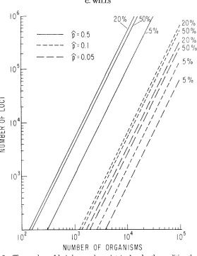
Figure 2 shows the numbers of loci that fit this criterion at each of several strengths of selection and selective equilibria.

For equilibria near 0.5, the ability of rank-order selection to maintain polymorphisms is very high. By extrapolating from Figure 2, it may be seen that for

(10)

412 c . WILLS

L L

[L w m

I

t

N U M B E R O F O R G A N I S M S

FIGURE 2.-The numbers of loci that can be maintained under the condition that up = $ / 5 for different numbers of organisms, different strengths of truncation and replacement, and different selective equilibria. Note that this is a log-log plot.

Nevertheless, even with 5% truncation and replacement and p^ = 0.05, as many as 66,000 polymorphic loci can be retained in a population of

lo5

individuals. If

selection is increased to 20%, this number reaches 330,000. These values can be compared with the estimate that there are 35,000 different poly-A-containing messages in a HeLa cell (BISHOP et aZ. 1974). If this estimate corresponds rough- l y to the number of translated genes in a higher eukaryote, then even if all of these are polymorphic with equilibrium frequencies near 0.05, rank-order selection still has the capacity to maintain additional untranslated polymorphism. An example of such polymorphism i s found in the spacer regions of Xenopus rRNA genes (REEDER et al. 1976), a function for which has not yet been determined.

(11)

RANK-ORDER SELECTION A N D POLYMORPHISM 41 3

the latter case increases the role of drift. It will be worthwhile, however, to ex- plore the possibility that this effect is due to the nature of the truncation, and might be avoided by other fitness distributions leading to identical changes in

H.

The chief element of uncertainty in these calculations involves the equating of N , with

N e .

N , is, however, the minimum pcjpulation size obtained each generation, and mating is at random, so that N e will exceed it, and these calculations will have overestimated the effect of drift.

MAGNITUDE O F SELECTION COEFFICIENTS

It will be seen from Figure 2 that the slopes of the lines are all two. The properties of truncation selection are such that the number of polymorphisms that can be maintained goes up as the square of the population size. FALCONER

(1960) showed that selection coefficients in truncation selection vary as an in- verse function of the standard deviation of the distribution. This is because truncation selection increases mean heterozygosity as a direct function of the standard deviation of the distribution.

This results in an enormous gain as the number of organisms increases, and is a general property of models in which selection acts on the standard deviation. Such models have been considered by SVED (1968) and MAYNARD SMITH (1968) from the standpoint of the substitution load. They showed that this type of selection reduces the substitution load to levels far lower than those calculated by

HALDANE (1957) on the basis of the multiplicative model. MAYNARD SMITH demonstrated that with 50% truncation of an infinite population in which a frequency of 0.9 was assigned to the less favorable allele at each locus, 71,000 loci could be acted upon by a selection differential of 0.01, compared to only 77 if

selection were multiplicative. If the selection coefficients are reduced tenfold to 0.001, then substitution in his formulas reveals that the permitted number of loci rises to over seven million in the truncation case, but increases only to 770 in the multiplicative case. Similarly, KING (1967) showed, for an infinite- population truncation model with a rigid threshold, that reducing the selection coefficient per locus by a factor of 10 reduced the proportion of variance due to overdominance by a factor of 100.

Another advantage of truncation models is that the selection coefficients associated with each locus can be relatively large. In the present model these coefficients are given by A p i / p i and A q i / q i , where the numerator is the change in p i and q i due to selection over one generation. For a given criterion governing the number of loci maintained, f o r instance our current criterion of up =

$/5,

(12)

414 c. WILLS

times the limit, and those associated with the commoner homozygotes are 45 times the limit.

These values remain constant for a given criterion for up, since varying the

selection intensity simply permits the maintenance of proportionately more or

fewer polymorphisms with the same strength of selection per polymorphism.

It is interesting to compare the magnitudes of the selection coefficients to be expected for rank-order selection and for strict multiplicative selection. I n the former case, the population size after selection,

N,,

is a function of the shape of the selection - curve; in the latter,

N 8 / N

=w.

Since when p” = 0.5, N , / N =

(1

-

s)L(l

-

H ) , the size of the selection coefficients in the multiplicative case

resulting in a given N , can easily be calculated.

Consider a population of size lo5, subject to

5%

truncation and replacement selection, which as we have seen can maintain about lo7 polymorphisms at p” = 0.5 when up = $/5. Here

N ,

is 9.5 X lo4 after truncation, and H i s approximately 0.5. Then under the multiplicative model, the average s will be

lo-*,

which is 250 times smaller than KIMURA’S lower limit. I n this case, the selection coefficients obtained from rank-order selection are 4,500 times as great as those obtained from the same amount of multiplicative selection. The differential becomes even greater for larger N .

DISCUSSION

An important limitation of the model considered in this paper is that the fitness curve imposed by the environment on the population stays approximately the same regardless of the values of the fitness potentials of the organisms making up the population. This is “pure” rank-order selection, and it assumes that environmental pressures are such that only a certain proportion of organisms survives, regardless of the value of the underlying fitness potentials. It is also pure “soft” selection as envisaged by

WALLACE

(1968). It seems likely, however, that most selection of functional polymorphisms falls between pure rank-order selection and multiplicative selection (the “hard” selection of WALLACE). I n such modified rank-order selection, the relative differences between fitness potentials determine to some degree the shape of the fitness curve imposed on the population. It seems reasonable to suppose, for example, that if a very great absolute difference exists between the most homozygous and the most heterozygous organism in a population, they will exhibit a larger fitness difference than they would if their hetero- zygosites were very similar. The extent of such an influence may be difficult to determine in practice, but in neither type of rank-order selection does the

absolute fitness potential value determine fitness directly, as it does in the multiplicative model.

(13)

RANK-ORDER SELECTION A N D POLYMORPHISM

A “ P U R E ” R A N K - O R D E R

I

B M O D I F I E D R A N K - O R D E R

41

5

2

m m w z

ti

L L

U C T C D n 7 V C n C I T V U F T E Dn7 Y C n C I T V /

l

I I

I I

HETEROZYGOSITY HETEROZYGOSITY

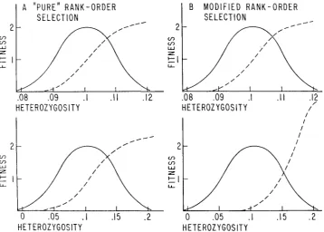
FIGURE 3.-Diagrams contrasting pure and modified rank-order selection. The solid lines show the distribution of heterozygosities in the selected populations, ranked from lowest“ to highest heterozygosity (which we take to be equivalent to “fitness potential”). The upper diagram in each set shows a population with a small variance of heterozygosity, and the lower diagram shows a population with a larger variance. The ordinate, in units of fitness, refers to the selection curve imposed on each population, which is shown by a dotted line and which is dependent on the stringency of the environment. In “pure” rank-order selection, represented in A, the shape of the fitness curve imposed by a particular environment does not alter as the variance of heterozygosity (fitness potential) changes. In modified rank-order selection, shown in B, as the variance of heterozygosity increases the intensity of selection also increases, giving a higher fitness t o organisms with an extremely high fitness potential. Thus, the differences between organisms on the fitness potential scale play a role in modified rank-order selection.

sult, for example, in a displacement of the fitness curve to the right. Modified rank-order selection is undoubtedly much more realistic, but much more difficult to handle analytically. It will be noted, however, that modified rank-order selection is influenced by the variance of heterozygosity. Factors such as linkage disequilibrium that change this variance will be considered in another paper.

(14)

416 c. WILLS

at the moment by the requirement that in each calculation all the loci be driven to the same selective equilibrium.

Finally, the calculations employed here are based on the assumption of un- conditional heterosis at every locus. An equilibrium population subject to such selection should have a distribution of allele frequencies very different from those actually observed in natural populations. Rank-order selection can maintain 150 times as many heterotic polymorphisms at a n equilibrium frequency of 0.5 as can be maintained at a frequency of 0.05. Thus, if polymorphisms with a variety of internal equilibria are constantly arising, the overwhelming majority of

those that are retained should be those with internal equilibria near 0.5.

I n fact, the distribution of allele frequencies in natural populations is U- shaped, and therefore the mirror image of what these calculations might lead US to expect. Indeed, this distribution of alleles forms the basis for powerful neutral- ist arguments (YAMAZAKI and MARUYAMA 1972). If, on the contrary, the majority of polymorphisms consist of functional alleles that are subject to selection, then the selection must be of a type that leads to an allele distribution mimicking the U-shaped one expected for neutrality. GILLESPIE (1977) has recently shown that this expectation is fulfilled for polymorphisms subject to randomly fluctu- ating selection pressures in which the heterozygote has approximately intermedi- ate fitness. Such polymorphisms are not being driven towards a single equilibrium. I t may be that a U-shaped distribution can also be derived from other selective models, such as for example models in which different types of selection are mixed. More information is therefore needed on the type of selection acting to maintain the majority of polymorphisms in natural populations, particularly with regard to the strength of genotype-environment interactions and the extent to which polymorphisms exhibit partial dominance. Despite these difficulties, there appears to be no insuperable obstacle to the maintenance of most genetic variability by selection.

I thank ROBERT A. ARMSTRONG, MICHAEL GILPIN and MICHAEL SOULB fo r discussions. Special thanks go to ROGER MILKMAN for endless patience and help. Supported by grant GM 19967 from the Public Health Service.

LITERATURE CITED

BERNSTEIN, S., L. H. THROCKMORTON and J. L. HUBBY, 1973

BISHOP, J. P., J. G. MORTON, M. ROSBASH and M. RICHARDSON, 1974

COYNE, J., 1976

FALCONER, D. S., 1960

FELSENSTEIN, J., 1976

Ann. Rev. Genet. 10: 253-280.

FLATZ, G., C. PIK and S. SRINGAM, 1965

Still more genetic variability in

Three abundance classes natural populations. Proc. Natl. Acad. Sci. U.S. 7 0 : 3928-3931.

i n HeLa cell messenger RNA. Nature 250: 199-204.

by varied techniques. Genetics 84.: 593-607.

Lack of genic similarity between two sibling species of Drosophila as revealed

Introduction to Quantitative Genetics. Oliver and Boyd, Edinburgh.

The theoretical population genetics of variable selection and migration.

(15)

RANK-ORDER SELECTION AND POLYMORPHISM

41

7

Sampling theory for alleles in a random environment. Nature 266: 443-446.

Overdominance and U-shaped gene frequency distributions. Nature 263 : 479-480.

A mathematical theory of natural and artificial selection. Part V. Selection and mutation. Proc. Camb. Phil. Soc. 23: 838-844. -

,

1957 The cost of

natural selection. J. Genet. 57: 51 1-524.

Enzyme polymorphism and adaptation. Stadler Genet. Symp. 7: 91-116. Genetic variability maintained in a finite population due to mutational production of neutral and nearly neutral isoalleles. Genet. Res. 11: 247-269. 1971 Theoretical foundations of population genetics at the molecular level. Theoret. Pop. Biol.

2: 174-208. GILLESPIE, J., 1977

GILPIN, M. E., M. S o u ~ k , A. ONDRACEK and E. A. GILPIN, 1976

HALDANE, J. B. S., 1927

JOHNSON, G. B., 1975

KIMURA, M., 1968

-

,

KING, J. L., 1967

LEWONTIN, R. C. and J. L. HUBBY, 1966 A molecular approach to the study of genic heterozygosity in natural populations. 11. Amount of variation and degree of heterozygosity in natural populations of Drosophila pseudoobscura. Genetics 54: 595-609.

MAYNARD SMITH, J., 1968 “Haldane’s Dilemma” and the rate of evolution. Nature 219: 11 14-1 116.

MAYR, E., 1959 MILKMAN, R. D., 1967

OHNO, S., 1972

REEDER, R. H., D. D. BROWN, P. K. WELLAUER and I. B. DAWID, 1976 Patterns of ribosomal DNA spacer length are inherited. J. Mol. Biol. 105: 507-516.

SAMPSELL, B., 1977 Isolation and genetic characterization of alcohol dehydrogenase thermo- stability variants occurring in natural populations of Drosophila melanogaster. Biochem. Genet. 15: 971-988.

The study of genic variation by electrophoretic and heat denaturation techniques at the octanol dehydrogenase locus in

members of the Drosophila virilis group. Genetics 8 0 : 637-650.

SINGH, R. S., R. C. LEWONTIN and A. A. FELTON, 1976 Genetic heterogeneity within electrophoretic “alleles” of xanthine dehydrogenase in Drosophila pseudoobscura. Genetics 84:

609-629. SVED, J. A., 1968

SVED, J. A., T. E. REED and W. F. BODMER, 1967 The number of balanced polymorphisms that

TOBARI, Y. N. and K. KOJIMA, 1967 Selective modes associated with inversion karyotypes in

WALLACE, B., 1968 Topics in Population Genetics. Norton, New York. __

,

1975 Hard

WILLS, C., 1973

YAMAZAKI, T. and T. MARUYAMA, 1972 morphism. Science 178: 56-58.

Continuously distributed factors affecting fitness. Genetics 55: 483-492.

Where are we? Cold Spr. Harb. Symp. Quant. Biol. 24: 1-14.

Heterosis as a major cause of heterozygosity in nature. Genetics 55:

493495. -, 1973 A competitive selection model. Genetics 74: 727-732.

So much “junk” DNA in our genome. Brookhaven Symp. Biol. 23: 366-370.

SINGH, R. S., J. L. HUBBY and L. H. THROCKMORTON, 1975

Possible rates of gene substitution in evolution. Amer. Nat. 102: 283-293.

can be maintained in a natural population. Genetics 55: 469-481.

Drosophila ananasscre. I. Frequency dependent selection. Genetics 57: 179-1 83. and soft selection revisited. Evolution 29 : 465-473.

In defense of naive pan-selectionism. Amer. Nat. 107: 23-34.

Evidence for the neutral hypothesis of protein poly-