Schurkus, Henry F. (2017): Highly Accurate Random Phase Approximation Methods With Linear Time Complexity. Dissertation, LMU München: Fakultät für Chemie und Pharmazie

Dissertation zur Erlangung des Doktorgrades

der Fakult¨at f¨

ur Chemie und Pharmazie

der Ludwig-Maximilians-Universit¨at M¨

unchen

Highly Accurate

Random Phase Approximation Methods

With

Linear Time Complexity

. . .

Henry Franz Schurkus

aus

Dissertation zur Erlangung des Doktorgrades

der Fakult¨at f¨

ur Chemie und Pharmazie

der Ludwig-Maximilians-Universit¨at M¨

unchen

Highly Accurate

Random Phase Approximation Methods

With

Linear Time Complexity

Henry Franz Schurkus

aus

Landshut

i

Erkl¨arung

Diese Dissertation wurde im Sinne von _§7 der Promotionsordnung vom 28.

Novem-ber 2011 von Herrn Prof. Dr. Christian Ochsenfeld betreut.

Eidesstattliche Versicherung

Diese Dissertation wurde eigenst¨andig und ohne unerlaubte Hilfe erarbeitet.

M¨_{unchen, . . . .}

. . . . (Henry Schurkus)

Dissertation eingereicht am _{. . . .}07.07.2017

1. Gutachter _{. . . .}Prof. Dr. Christian Ochsenfeld

2. Gutachter _{. . . .}Prof. Dr. Hubert Ebert

iii

Summary

One of the key challenges of electronic structure theory is to find formulations to compute electronic ground-state energies with high accuracy while being applicable to a wide range of chemical problems. For systems beyond the few atom scale often computations achieving higher accuracies than the so called double-hybrid density functional approximations become prohibitively expensive. Here, the random phase approximation, which is known to yield such higher accuracy results has been developed from a theory applicable only to molecules on the tens of atoms scale into a highly accurate and widely applicable theory. To this end, a mathematical understanding has been developed that, without changing the computational complexity, allows to eliminate the error introduced by the resolution-of-the-identity approximation which had been introduced in the previous formulation. Furthermore, in this work a new formulation of the random phase approximation for molecules has been presented which achieves linear-scaling of compute time with molecular size—thereby expanding the realm of molecules that can be treated on this level of theory to up to a thousand atoms on a simple desktop computer. Finally, the theory has been matured to allow for use of even extensive basis sets without drastically increasing runtimes. Overall, the presented theory is at least as accurate and even faster than the original formulation for all molecules for which compute time is significant and opens new possibilities for the highly accurate description of large quantum chemical systems.

List of publications

The present work is a cumulative dissertation, comprising three publications in peer-reviewed journals. The content of these is given completely in chapter 3 together with supporting information that was published conjointly.

I “An effective linear-scaling atomic-orbital reformulation of the random-phase ap-proximation using a contracted double-Laplace transformation”,

H. F. Schurkus and C. Ochsenfeld,

J. Chem. Phys. (Communication) 144, 031101 (2016).

II “Vanishing-Overhead Linear-Scaling Random Phase Approximation by Cholesky

Decomposition and an Attenuated Coulomb-Metric”, A. Luenser, H. F. Schurkus, and C. Ochsenfeld,

J. Chem. Theory Comput. 13, 1647 (2017).

Contributions by H. F. Schurkus: Conjoint development of the theory with A.

Luenser. Contributions to implementation and major contributions to writing.

III “Almost error-free resolution-of-the-identity correlation methods by null space removal of the particle-hole interactions”,

H. F. Schurkus, A. Luenser, C. Ochsenfeld,

J. Chem. Phys. (Communication) 146, 211106 (2017).

Contributions by H. F. Schurkus: Conjoint development of the theory with A.

Luenser. Development of the mathematical basis of the theory and derivation of the equations. Most of the calculations and writing. Contributions to implemen-tation.

Contents

1 Introduction 1

2 Theoretical Basics 5

2.1 Overview of Electronic Structure Theory . . . 5

2.2 Computational Complexity . . . 6

2.2.1 Asymptotic and Effective Time-Complexity . . . 6

2.2.2 Measuring Time-Complexity . . . 9

2.3 Resolution-Of-The-Identity . . . 10

2.3.1 Overlap Metric Resolution-Of-The-Identity of Electron Repul-sion Integrals . . . 10

2.3.2 Density Fitting . . . 13

2.4 Random Phase Approximation . . . 14

2.4.1 Important Results from Green’s Function Theory . . . 14

2.4.2 Adiabatic Connection . . . 18

2.4.3 Polarization Propagator and Random Phase Approximation . . 20

2.4.4 Evaluation of iΠ0 by Lehmann’s Representation . . . 23

2.4.5 Molecular Orbitals . . . 26

3 Publications 29 3.1 AO-RI-RPA . . . 29

3.2 ω-CDD-RPA . . . 39

3.3 Kernel Projection . . . 51

4 Conclusion 75

Chapter 1

Introduction

The field of theoretical chemistry is concerned with the theoretical description and prediction of atomic and molecular processes. To this end it is crucial to describe the electronic structure—including the quantum nature of electrons. It can be proven1_that

finding the exact solution for the Schr¨odinger equation for a general system of electrons is of the Quantum-Merlin-Arthur2 _{complexity class, making it highly unlikely that it}

could be done without approximation. As the electronic Schr¨odinger equation3 _already

neglects all relativistic effects,4 _{even further approximations are necessary. Therefore}

a large part of electronic structure theory is concerned with the development of such approximations yielding numerically accurate results for a broad range of molecules.

One approximation to compute the electronic ground state in a fixed field of nuclei which has received a lot of attention in recent years is the random phase approximation5

(RPA). It can be shown to be far more accurate than the frequently employed density functional approximations (DFAs; e.g. the widely used B3LYP functional6_{), Hartree–}

Fock theory,7–10 _{and Møller–Plesset perturbation theory}11 _{(MP2). A more detailed}

discussion of where RPA fits into the bigger picture of electronic structure theory can be found in Sec. 2.1.

The RPA was originally conceived in work by Bohm and Pines5 _{in 1953, but has}

long been of little use to theoretical chemistry because its computational complexity limited its application to systems of a few atoms. For such systems, however, coupled cluster theories12, 13 _{can also be applied, which would yield even better accuracies in}

comparison. This changed in 2010, when Furche and coworkers developed a theory combining the RPA with the resolution-of-the-identity14–18, 33_{(RI) to achieve an overall}

scaling with molecular size of O(M4_log(M)).19 _{It allowed to apply their theory}

(RI-RPA) to systems of several tens of atoms—far beyond what is viable with accurate coupled cluster theories, yet still very limited. In Sec. 2.4 a more thorough elaboration on the RPA theory leading up to the present work can be found.

coming years.

In the first publication of this work a different formulation or more specifically metric of the RI than the Coulomb metric of RI-RPA is applied and a new inte-gral transformation, called double-Laplace, related to the Laplace transform in linear

scaling AO-MP2 theory20 _{is derived. Combined, double-Laplace and the different RI}

metric allow to formulate a theory that achieves the same level of accuracy as RI-RPA but scales only linearly with molecular size. This theory can therefore be applied to

molecules of up to a thousand atoms and ten thousand basis functions.21 _{To achieve}

linear-scaling behavior, the new theory exposes and exploits the physical locality of electron correlation within the random phase approximation. To this end it is based on (pseudo) density matrices in the atomic orbital (AO) basis and titled AO-RI-RPA. A more detailed discussion of RI and the related concept of density-fitting22 _{(DF) can}

be found in Sec. 2.3.

While the number of electrons scales only with system size, the number of atomic orbitals also scales with basis set size. Therefore, while AO-RI-RPA allows to compute systems untractable with RI-RPA due to their sheer size, for any fixed size molecule increasing the basis set size raises the computational cost of AO-RI-RPA faster than in the case of RI-RPA. This is remedied in the second publication of this work, where a Cholesky decomposition of the density matrices23–25 _{(CDD) is introduced. The}

tech-nique had been explored in the context of AO-MP2 where the Laplace transform gives rise to one kind of pseudo density matrix. In this publication it was extended to also treat the second kind which stems from the new integral transform of AO-RI-RPA. With CDD the presented theory can then be denoted by CDD-RI-RPA and the scaling with basis set size is again the same as with RI-RPA, while at the same time CDD-RI-RPA still allows for linear scaling evaluation and therefore the computation of even larger systems than the previous AO-RI-RPA. With CDD-RI-RPA, converging results with basis sets of quadruple-ζ size becomes standard practice even for systems with several hundreds of atoms.26

While the so called overlap metric RI was introduced in formulating AO-RI-RPA, the Coulomb metric is more commonly used in other theories as for example in DF-DFT and RI-MP2.27 _{Accordingly, the auxiliary basis sets necessary for evaluation of}

the RI are mostly optimized and published for the Coulomb metric.28–32 _{Also, it has}

been shown that the Coulomb metric is optimal for evaluation of the energy at least in the case of DF-DFT.33 _{For this reason the second publication of this work furthermore}

develops the RI metric further. The core feature of the overlap metric that gives rise to the option of linear scaling in AO-RI-RPA is its locality. By introducing an attenuated Coulomb metric which has tunable locality, the best of both worlds can be combined:26 _{The final ω-CDD-RPA theory allows for linear-scaling evaluation while at}

the same time results are identical to those obtained with Coulomb metric RI within numerical accuracy.

As indicated above, the RI is formally exact when the size of the auxiliary basis set tends to completeness. Preoptimized auxiliary basis sets28–32_{employed in practical}

calculations, however, are typically only about three times larger than the AO basis set. This is generally justified by the concept of DF and allows to reduce computational cost by a significant factor.14, 22, 33 _{However, this procedure also drastically deteriorates}

3

modification of the RI scheme that still achieves evaluation times comparable to those of using standard preoptimized auxiliary basis sets.

To this end a new concept has been developed in the third publication, designated nullspace projection. Nullspace projection describes a procedure to project out the nullspace of an arbitrary operator chain and thereby reduce the matrix dimensions at the boundaries of the chain. It is shown that the physical-model operator of RPA in auxiliary basis representation is of limited rank and therefore nullspace projection allows to reduce the number of auxiliary basis functions without introduction of any error. By employing a converged auxiliary basis set and nullspace projecting the phys-ical model, the error of the RI is de-facto eliminated for only slightly more compute time than with standard preoptimized auxiliary basis sets.71

Chapter 2

Theoretical Basics

In this chapter the theoretical basis of the original research of chapter 3 is summarized. First, in Sec. 2.1, an overview of the field of electronic structure theory is given and the accuracy of the RPA contrasted with other approximation theories. In Sec. 2.2 important aspects of defining and measuring the computational cost of approximation theories are discussed. Computational costs limit the applicability of a theory and one of the key aspects of the research presented in chapter 3 is the dramatic reduction of cost for the RPA. In Sec. 2.3 the RI in overlap metric and Coulomb metric is introduced and the source of error of employing RI in approximation theories is discussed. The RI is a major theme of the publications of the following chapter, as the first two publications employ a change of metric to allow for a computationally efficient theory without deteriorating accuracy and the third publication develops a scheme to eliminate the error introduced by the RI completely for only slightly increased computational cost. Finally, in Sec. 2.4, a concise derivation of the RPA for molecular systems is presented. Although historically a more cumbersome derivation formed the basis of the first publication of chapter 3, it can be understood directly from this result obtained in a more physically motivated way.

2.1

Overview of Electronic Structure Theory

As stated in the introduction, the goal of electronic structure theory is the develop-ment of approximations that make evaluation possible and feasible for a wide range of molecules without diverging unnecessarily from the exact solution.

One approximation so common that it is often not even considered an approxima-tion is the use of finite predefined basis sets28–32 _{to discretize the differential equations}

of quantum mechanics into a linear algebra of vectors, matrices, and higher order ten-sors. While for other applications different types of basis sets have proven useful—e.g. plane waves as the basis for calculations of periodic systems72, 73_{—for molecular}

sys-tems atom-centered Gaussian type functions have been established as the predominant choice.

Theories that do so purely from mathematical concepts are calledab initio. Within these there exists a strong order from highly accurate but computationally expensive to much less demanding but also less accurate theories. For the few atom regime cou-pled cluster theories12, 13 _{(CC) are available, for larger molecules perturbation theories}

like second-order Møller–Plesset theory11 _{(MP2) can be applied and for the largest}

molecules one is often restricted to Hartree–Fock theory7–10 _{(HF) in practice.}

By introduction of empirical parameters often better quality results for the same

expense as with ab initio theories can be achieved. This path is mainly explored

with Kohn–Sham density functional theory41 _{(DFT) which is in contrast to ab initio}

theories sometimes also referred to as first-principles. DFT reformulates the problem by mapping the interacting system of electrons to a model system of non-interacting electrons. While this mapping can in principle be made exact, the necessary exact density functional is in general unknown and so it is necessary to introduce density

functional approximations (DFAs). These often incorporate contributions from ab

initio theories because those are already considered very accurate. The contributions

fromab initio theories are then weighted by empirical factors together with other purely

density based contributions. The DFAs can be grouped by the ab initio contributions

they incorporate.42 _{DFAs that depend solely on the density can already describe}

the Coulomb interaction of electrons exactly and are known as (semi-)local DFAs. Hybrid DFAs additionally contain the so-called exact exchange contribution from HF theory. Lastly, double-hybrid DFAs additionally incorporate a contribution to the correlation energy as described by MP2 theory. While most DFAs aim to keep the

number of weighting parameters low, also DFAs with hundreds of parameters exist.43

The downside to these empirical parameters is that the order between the levels of theory becomes less rigorous as chances increase that the lower level of theory may be right for the wrong reason.44

Most DFAs describe electron densities rather well and so the adiabatic connection45

allows to formulate a perturbation theory on the electron density or equivalently the Kohn–Sham orbitals obtained from a DFA that in principle converges to the exact solu-tion. Within this series again approximations can be introduced. The most prominent

of these is the random phase approximation5 _{(RPA). The RPA neglects certain terms}

of the perturbation series but includes others exactly to infinite order. It is therefore rather robust against the choice of DFA with which the initial density is computed and also size-consistent. Energies are typically much better than those obtained with the different DFAs, HF or MP2, however not quite as good as those of coupled clus-ter theory with singles, doubles and perturbative triples contributions74 _(CCSD(T))

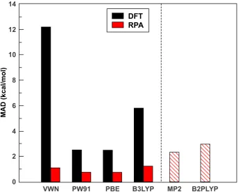
which remains the gold standard for highly accurate computations. A comparison of energies obtained with different DFAs and RPA calculations based on these DFAs ref-erenced against this gold standard has previously been presented by the author.46 _It

is reproduced below for illustration (Fig. 2.1).

2.2

Computational Complexity

2.2.1

Asymptotic and Effective Time-Complexity

2.2. COMPUTATIONAL COMPLEXITY 7

M

A

D

(

kc

al

/m

o

l)

0 2 4 6 8 10 12 14

VWN PW91 PBE B3LYP MP2 B2PLYP

DFT RPA

limited by the compute time necessary to evaluate the theory. When compute time requirements go beyond a few weeks for a single calculation they become practically unfeasible. On the one hand, because often the result of one calculation informs the configuration of the next and therefore research projects quickly require intolerable amounts of time. On the other hand, todays computers may malfunction or require intervention over a time scale of several weeks when put under heavy load and keeping calculations running much longer can therefore require significant effort.

Computational complexity denotes the time required for evaluation of an algorithm as a function of the problem size. As different problems of equal size may take differing time to compute by an algorithm one typically considers worst-case time complexity. The specific form of the time complexity function may be very involved. However, to estimate for which size of molecules runtime becomes limiting, it is often sufficient to

approximate its limit by a polynomial. The Bachmann-Landau notation47, 48 _{is used}

throughout computer science to formalize this process. According to this notation a functiont(M) is associated with a polynomial poly(M) as

t(M)M=→∞O(poly(M))

:⇐⇒

∃ const_∈R, M0 ∈R: ∀M ≥M0 : |t(M)| ≤const· |poly(M)| . (2.1)

In words, a time complexity is _O(poly(M)) exactly when for all systems of larger size than a certain size M0 the evaluation time is smaller than a constant times this polynomial poly(M).

It has been argued that electrons in many-atom systems express “nearsighted-ness”,49 _{so that different potentials or densities beyond a certain distance have only}

limited effect on local electronic structure.50 _{On this basis it seems plausible, that for}

any approximation theory that captures the physics of the electronic system correctly, there should exist a linear-scaling formulation.

How such a reformulation can be found is however in general not clear. To develop a linear-scaling theory without introducing additional approximations it is necessary to expose the physical locality that is hidden in the canonical formulation of the theory. It then has to be exploited by circumventing computational steps that due to this locality would yield only vanishing contributions to the final result.

Given thede facto time limit discussed above, the order of magnitude of molecular sizes treatable with a given theory is mainly dependent on the order of the asymptotic polynomial with molecular size M, because different prefactors are quickly overshad-owed by any difference in polynomial order when molecular size increases. When

com-paring compute times of moderately sized molecules (where M is comparably small)

or different algorithms of equal polynomial order, however, these prefactors can play a significant role in determining evaluation time.

2.2. COMPUTATIONAL COMPLEXITY 9

complexity with N is often of similar but not necessarily equal order as that with M. Even more subtle analyses can be made, when also auxiliary basis set sizeNaux is taken into consideration (which is otherwise simply taken as proportional toN) and instead of molecular sizeM—which doesn’t discriminate between light and heavy atoms in the molecule—the number of electrons Nel is used.

Up to this point the asymptotic limit, Eq. 2.1, has been taken in discussing limiting compute time. One sometimes finds that certain steps of an algorithm may by asymp-totically dominating but are not even detectable in actual runtime measurements, or timings for short. This may be caused by orders of magnitude lower prefactors of the corresponding steps in comparison to the other steps of the overall algorithm. In these cases it is more suitable to discuss effective scaling behavior than asymptotic scaling behavior, which means that the limit is taken not to theoretical infinity but to the largest molecules which can in fact be treated by the theory.

RI-RPA scales effectively _O(M4_{) with molecular size and O(N}3_{) with basis set}

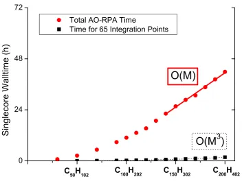
size. The high order scaling with molecular size strongly constrains its applicability to molecules of limited size. AO-RI-RPA, which is presented in the first publication of this work, lowers the effective scaling with molecular size from _O(M4_{) to O(M)}

enabling its application to much larger systems. Because it also raises scaling with basis set size from O(N3_{) to O(N}4_{), however, for small molecules or computations}

with large basis sets the RI-RPA evaluates faster. With CDD-RI-RPA, as presented in the second paper of this work, the effective scaling with molecular size is still_O(M) but with basis set size it is again reduced toO(N3_{) so that it evaluates faster than}

RI-RPA even for medium sized molecules. Only for the very smallest of molecules, where the description of the actual time complexity is not yet described by the polynomial, Eq. 2.1, CDD-RPA is sometimes observed to take more time to evaluate than RI-RPA. This is of no concern however, because for these very small molecules absolute evaluation times are in the range of a few minutes or even less.

2.2.2

Measuring Time-Complexity

Different measures have been considered to analyze the time complexity of real im-plementations of quantum chemical theories. The most straightforward approach to approximate the order of the polynomial is by considering a systematically enlargable model system. Ideally this is a system of molecules, such that when a molecule with an x-fold number of atoms is chosen also every other extensive parameter is scaled x -fold: the number of basis functions, electrons, and physical interactions. This means, that the molecule should be of linear shape, because otherwise the number of physi-cal interaction cannot be proportional to the number of electrons. Furthermore, the molecules should be built from repeating building blocks and either have no bound-aries or boundbound-aries with negligible effects. A good tradeoff between chemical realism and these requirements which can never be fulfilled by any truly realistic system to arbitrary size, is the system of linear alkanes. They are built up from repeating -CH2

physi-cal interactions would get entangled with the time-complexity of the implementation under scrutiny.

A gross estimate of the time complexity can be made with such systematically enlargable molecules by considering two molecules, one of double the size of the other, and comparing their respective compute times. If they differ by a factor of two as well, the implementation is said to be linear, if the factor is four, the implementation is quadratic, and so on. This is equivalent to fitting t(M) for the two molecules by a monomial with adjustable exponent and dropping the coefficient afterwards. The smallest system size for which a certain order is found in this way is then considered the onset of that asymptotic time complexity.

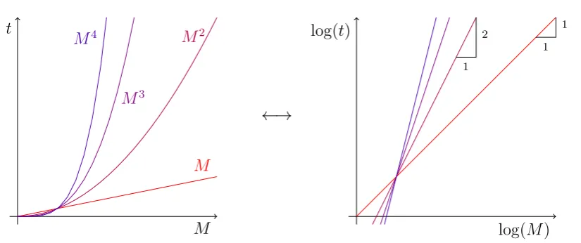
A more accurate representation of Eq. 2.1 is illustrated in Fig. 2.2 and can be given as follows: The largest molecules are fitted by

f(M) = mono(M)−∆ (2.2)

where mono(M) is again a monomial and ∆ is a variable positiveM-independent offset. Then mono(M) is always larger than the fit f(M) and therefore larger than t(M) for the fitted molecule sizes and Eq. 2.1 is fulfilled for all sizes in the fitting range. The coefficient can be dropped again or the whole monomial taken as the asymptotic time complexity. The smallest size for which a fit with this size as the lower end of the fitting range is well justified can be taken as the onset of the corresponding time complexity. To fit Eq. 2.2 and also for better clearness of display it is sometimes useful to plot double logarithmically (Fig. 2.3). For monomials cMx _{this leads to straight lines with} slopex and offset log(c)/log(M). In ranges where actual time complexity is very close to a monomial the order of the polynomial can therefore be read off a graphical display with ease and fitting is more robust in cases where the scaling is not linear.

2.3

Resolution-Of-The-Identity

As all electronic structure theories aim to solve the Schr¨odinger equation,3 _{which is}

a differential equation, a major ingredient that appears in almost all electronic struc-ture theories are integrals containing basis functions and (differential) operators. The number of basis function indices, or centers, defines the order of the integral tensor. The higher this order, the higher the cost of computation and storage. Here, only real-valued basis functions will be considered. The resolution-of-the-identity14–18, 33 _is

an idea to reduce the number of centers that occur in an integral by replacing a single integral with tensor products of multiple integrals of lower order.

2.3.1

Overlap Metric Resolution-Of-The-Identity of Electron

Repulsion Integrals

The most prominent example of RI is its use in the context of electron repulsion integrals (ERIs), here in Mulliken notation

(µν_|Vˆee|λσ) =

ZZ

dxdx0 χµ(x)χν(x)Vee(x,x0)χλ(x0)χσ(x0) . (2.3)

If the operator in the integral is the electron interaction operator

Vee(x,x0) = 1

2.3. RESOLUTION-OF-THE-IDENTITY 11

M t

O(M)

mono(M) =M

fitting region

∆

Figure 2.2: The effective scaling of an algorithm can be found by fitting the largest measured runtimes by Eq. 2.2. In this qualitative illustration the runtime behaves in a complex way up until a point when the behavior becomes essentially linear. A linear fit through all points from this point onwards predicts all points perfectly but does not pass the origin due to the complex behavior for small systems. For this reason the more simple approach fails. Shifting the fit line up by ∆ however always overestimates the true runtime and is still linear. According to the Bachmann-Landau notation it is therefore O(M).

←→

M t

log(M) log(t)

M

M2

M3

M4 1

1 2

1

the symbol can be dropped by convention

(µν_|Vee|λσ)≡(µν|λσ) . (2.5)

In this section Einstein’s sum convention is employed, which states that indices that appear twice in any term are implicitly summed over.51 _{This drastically}

simpli-fies notation of tensor contractions. As an example, for tensors of second order, i.e. matrices, the (µ, ν)-th element of the product of two matrices is simply given by

(AB)µν =Aµ,κBκ,ν . (2.6)

Matrix operations are to be taken before indexing in this work, e.g., the (µ, ν)-th element of the inverse of (µν) is written as (µν)−1_.

A complete orthonormal set of states _|Φni is defined as fulfilling

1 =|Φni hΦn| (2.7)

Introduction of this resolved identity between the operator and the basis functions in Eq. 2.3 yields

(µν|λσ) = (µνn)(n|m)(mλσ). (2.8)

The two and three center integrals here are in consistence with Eq. 2.3 defined as

(µνm) =

Z

dxχµ(x)χν(x)Φn(x) (2.9)

(n|m) = Z

dxdx0 Φn(x)Vee(x,x0)Φm(x0) . (2.10)

Since the RI is introduced only in the vicinity of basis function products |µν), it is not necessary for Eq. 2.7 to represent a general identity over all space, but only over the subspace representable by such products. For Gaussian type basis sets

χµ(x) =xmµynµzlµe−ζµ|x−Rµ|

2

(2.11)

any such product is again a sum of Gaussian type functions because

e−ζµ|x−Rµ|2_e−ζν|x−Rν|2 _=Ke−ζ|x−R|2 _(2.12)

where

K = eζ|R|2−ζµ|Rµ|2−ζν|Rν|2 _(2.13)

R = ζµRµ+ζνRν

ζ (2.14)

ζ = ζµ+ζν (2.15)

as can be seen by multiplication and comparison of the coefficients.

2.3. RESOLUTION-OF-THE-IDENTITY 13

Unfortunately, Gaussian type functions are not orthogonal to one another and so cannot fulfill Eq. 2.8. From a complete set of Gaussian type functions, or auxiliary (ba-sis) functionsχP as they will be called from here on, however, a complete orthonormal set can be constructed by L¨owdin orthonormalization52–54

|ΦPi=|χQi hχQ|χPi−1/2 . (2.16)

Insertion of Eq. 2.16 into Eq. 2.7 then yields for Eq. 2.8

(µν|λσ) = (µνP)(P Q)−1(Q|R)(RS)−1(Sλσ) (2.17)

For Eq. 2.17 to hold as an identity it is necessary for the auxiliary basis to be complete. To facilitate evaluation the auxiliary basis is typically taken to be atom-centered just as the regular basis set. It is then necessary to take very large auxiliary basis sets to still ensure completeness. Otherwise, Eq. 2.17 weakens to an approximation.

2.3.2

Density Fitting

An alternative derivation shows why such an approximation is viable. If two indices of the ERI are contracted with the density matrix, a matrix is obtained that represents the Coulomb interaction of a basis function pair with the charge density of all electrons

Jµν = (µν|ρ) = (µν|λσ)Pλσ (2.18)

as it occurs in Hartree–Fock theory and Kohn–Sham DFT. The product pair can therefore be seen as a generalized density ρλσ. Fitting this density with an incomplete set of auxiliary functions28–32 _{with coefficients c}λσ

P

|λσf) = cλσ_p |P) (2.19)

results in a deviation

∆ρλσ =|λσ)− |λσf) (2.20)

which can be minimized by an appropriate choice of the coefficients.14

As the deviation is, however, still a function of space, a choice of metric has to be made to fold it into a single value which can then be minimized analytically. One approach is to take the overlap metric33 _{and therefore deduce}

0 =! ∂

∂cλσ P

(∆ρµν∆ρλσ) (2.21)

= ∂

∂cλσ P

(∆ρµν ρλσ)−(∆ρµνP)cλσP

(2.22)

= ₋(∆ρµνP) (2.23)

= ₋ (µνP)₋cµν_Q (QP) (2.24)

cµν_Q = (µνP)(P Q)−1 (2.25)

resulting in

(µν|λσ)≈(µνf|λσf) = (µνP)(P Q)−1(Q|R)(RS)−1(Sλσ) . (2.26)

Another metric which has been found to be optimal33_{for the evaluation of Eq. 2.18}

is the choice of Coulomb metric

0=! ∂

∂cλσ P

(∆ρµν|∆ρλσ) (2.27)

which accordingly leads to

(µν_|λσ)_≈(µν_f|λσf) = (µν_|P)(P_|Q)−1(Q_|λσ) . (2.28)

The fitting approach applies in this form only to the special case of ERIs. It has been argued for the final equation to be identified as density fitting (DF) instead of RI.22

In the third publication of this work the derivation is carried out with the attenuated Coulomb metric in mind and it is shown in the accompanying supporting information that Eq. 2.28 can also be derived from the point of view of RI by expressing the complete orthonormal basis again in a complete non-orthogonal basis. The essential difference between RI and DF is then, that the RI can also be found in more general contexts and argues from the point of view of complete basis sets while the DF is mostly restricted to ERIs and argues from the point of incomplete basis sets.

2.4

Random Phase Approximation

The RPA5 _{can be derived within different contexts of electronic structure theory. Here,}

a derivation is given that employs Feynman–Dyson perturbation theory55–58_{also known}

as Green’s function theory, for which Fetter and Walecka have written a very

compre-hensive account.59 _{The essential results of Feynman–Dyson perturbation theory are}

restated in Sec. 2.4.1 and the RPA is rigorously derived from these in the succeeding sections.

2.4.1

Important Results from Green’s Function Theory

Second Quantization

Kohn–Sham DFT constructs a Fock operator ˆFKS, so that the sum of squared

eigen-functionsϕp, fulfilling

ˆ

FKSϕp(x) = εpϕp(x) (2.29)

reproduces the exact density of the interacting system

n(x) =X i

|ϕi(x)|2 (2.30)

The orbital energiesεp can generally be sorted in non-descending order and the indices [1, . . . , Nel] are called occupied and all others unoccupied or virtual. Here and through-out this work sums overp, q, . . . run over all indices,i, j, . . . over the occupied indices, and a, b, . . . over the virtual indices. Also, Einstein’s sum convention51 _{is generalized}

2.4. RANDOM PHASE APPROXIMATION 15

The one particle Fock eigenfunctions ϕp can be combined into antisymmetrized

products, called Slater determinants60 _{that are then N}

el-particle functions

hx1x2· · ·xNel|ϕpϕq· · ·ϕri:=

1

Nel!

1/2

ϕp(x1) · · · ϕp(x1)

... . .. ...

ϕr(xNel) · · · ϕr(xNel)

(2.31)

To derive a correction to the Kohn–Sham DFT result it is useful to describe the theory in the basis of Slater determinants—which combined cover the space of all an-tisymmetrized wavefunctions. The non-relativistic second quantization formalism62–64

allows for a particularly straightforward derivation of the following results. In sec-ond quantization each Slater determinant is associated with a Fock state, which is an eigenstate of the number operator

ˆ

np = ˆa†pˆap (2.32)

where ˆa†

p is the creation operator for the p-th one-particle function and ˆap the cor-responding annihilation operator. The mode operators ˆa† and ˆa are defined by the canonical anticommutation relations

{ˆap,ˆa†q} = δpq (2.33)

{ˆap,ˆaq} = {ˆa†p,ˆa†q}= 0 (2.34)

and can further be linearly combined into field operators

ˆ

ψ(x) = ϕp(x)ˆap (2.35)

to allow for formulations in real space instead of mode space. This also allows for a very simple description of operators in second quantization, by integration of their matrix elements in space-representation with the corresponding field creation operators to the left and field annihilation operators to the right, e.g.

ˆ

Vee= ˆψ†(x) ˆψ†(x0)Vee(x, x0) ˆψ(x0) ˆψ(x) . (2.36)

Interaction Picture

The exact ground state of the full interacting Hamiltonian ˆH is defined by

ˆ

H_|Ψ_i=E_|Ψ_i . (2.37)

In the Schr¨odinger picture the states|Ψ(t)iare time-dependent. Only in the Heisenberg picture, where all time-dependence is shifted to the operators can Eq. 2.37 truely be considered the time-independent Schr¨odinger equation. Because the time-dependence can be expressed by an operator that is due to the Hamiltonian and therefore trivially commutes with it, the time-dependence of ˆH vanishes. As Eq. 2.37 can in general not be solved exactly, one resorts to

ˆ

H0|Φi=E0|Φi (2.38)

where ˆH0 is given by

ˆ

with the one-particle operator ˆh and the Kohn–Sham potential v, so that |Φi is the ground state Slater determinant. _|Φ_i is only time-independent in a universe that is completely described by ˆH0—a universe in which all particles are non-interacting. In a universe that is described by ˆH, however, |Φi develops with time.

The interaction picture shifts only the time-dependence due to ˆH0 into the operators

and keeps the other time-dependence due to the then time-dependent interaction ˆ

H1(t) := ˆH(t)−Hˆ0 (2.40)

with the state. The state then propagates due to the time propagation operator61

ˆ

U(t, t0)

|Φ(t)_i=: ˆU(t, t0)_|Φ(t0)_i . (2.41)

Gell-Mann–Low Theorem

The key idea to the Gell-Mann–Low theorem65 _{is to consider an adiabatic process of}

switching on the interaction ˆH1 in the universe adiabatically slowly ˆ

H = ˆH0+e−|t|H1ˆ , (2.42)

where is send to zero later. This means, that at finite times (around t = 0) the

universe behaves due to the physical, i.e. interacting, Hamiltonian ˆH. On the other hand, at infinitely early and late times the universe behaves according to the non-interacting Hamiltonian ˆH0 and the exact ground state is therefore known for these points in time. In this picture, the time propagation operator is explicitly obtained as

ˆ

U(t, t0) = ∞

X

n=0

(₋i)n

n! Z t

t0

dt1_{· · ·}

Z t

t0

dtnT

h ˆ

H1(t1)_{· · ·}H1ˆ (tn)

i

(2.43)

≡ The−i

Rt t₀dt

0_Hˆ

1(t0)i _(2.44)

with the time-ordering operation T [_{· · ·}]. A product of operators ˆO1(t) ˆO2(t0_{) is said to} be time ordered if t > t0 and the time-ordering operation permutes its argument into time order. Depending on the number of permutations the global sign changes under this operation.

With the time propagation operator defined by Eq. 2.44, the Gell-Mann–Low the-orem65 _{states that if}

lim →0

ˆ

U(0,±∞)|Φi

hΦ_|Uˆ(0,±∞)|Φi

≡ |Ψi

hΦ_|Ψ_i (2.45)

exists to all orders of perturbation theory, it is an eigenstate (usually the ground state) of the exact Hamiltonian.

ˆ

H |Ψi hΦ_|Ψ_i =E

|Ψ_i

hΦ_|Ψ_i (2.46)

Wick Theorem

To evaluate expectation values due to this interacting ground state it is useful to observe that for a Heisenberg operator ˆOH(t)

hΨ|OˆH(t)|Ψi

hΨ_|Ψ_i = 1 hΦ|Sˆ|Φi

X

n

(−i)n

n!

Z ∞

−∞· · ·

Z ∞

−∞h

Φ|ThH1ˆ (t1)· · ·H1ˆ (tn) ˆOI(t)

i |Φi

2.4. RANDOM PHASE APPROXIMATION 17

where

ˆ

S = ˆU(_∞,_−∞) (2.48)

and ˆOI is the same operator chain in the interaction picture. This result extends naturally when a time-ordered chain of operators is used instead of ˆOH(t).

Besides time-order introduced above, another useful order of operators is normal order, and N [_{· · ·}] is the corresponding normal-ordering operation. A chain of operators is said to be normal ordered if the _|Φ_i expectation value of it vanishes, so

hΦ_|NhOˆ1Oˆ2· · ·

i

|Φ_i= 0 . (2.49)

Combined the two ordering operations allow to define the contraction of two operators

ˆ

O1O2ˆ := T

h ˆ

O1O2ˆ i₋NhO1ˆ O2ˆ i (2.50)

While time ordering and normal ordering affect whole operator chains, each

con-traction affects only two operators. Wick’s Theorem66 _{thus allows to evaluate the}

time-ordered chain in Eq. 2.47 by stating that a time-ordered chain of operators is equal to the sum of normal-ordering of all possible contractions over the chain

ThO1ˆ O2ˆ O3ˆ _{· · ·}i = N "

ˆ

O1O2ˆ O3ˆ _{· · ·}

# + N

" ˆ

O1O2ˆ O3ˆ _{· · ·}

# +_{· · ·}

+ N "

ˆ

O1O2ˆ O3ˆ _{· · ·}

# +_{· · ·}

+ · · · (2.51)

Because the time-ordered product in Eq. 2.47 occurs between _|Φ_i, all incomplete con-tractions vanish trivially (cmp. Eq. 2.49). Wick’s theorem reduces the problem of evaluating an expectation value of the interacting ground state to summing up a series of terms consisting only of products of contractions.

Green’s Function

The most important contraction in second quantization is the non-interacting Green’s function, also called propagator,67–69 _{which is the contraction of a field destruction and}

field creation operator.

iG0(x, x0) := _hΦ_|Thψˆ(x) ˆψ†(x0)i_|Φ_i (2.52)

= hΦ|Thψˆ(x) ˆψ†(x0)i−Nhψˆ(x) ˆψ†(x0)i|Φi (2.53)

= hΦ|ψˆ(x) ˆψ†(x0)|Φi (2.54)

= ψˆ(x) ˆψ†(x0) (2.55)

The index zero denotes that the expectation value is to be taken with respect to _|Φ_i which is the non-interacting ground state of ˆH0. The interacting Green’s function is accordingly defined as

iG(x, x0) := h

Ψ_|Thψˆ(x) ˆψ†_(x0₎i_|Ψi

hΨ_|Ψ_i (2.56)

Feynman Diagrams

Eqs. 2.47 and 2.51 are still unwieldy to work with. To allow for a more accessible notation, Feynman put forward the idea of writing diagrams to represent the

respec-tive terms.55, 56 _{Each diagram consists of nodes and lines between them. The nodes}

correspond to points in space-time. A non-interacting Green’s function iG0(x, x0_{) is} represented by a curved or straight line with an arrow pointing from the x0 to the x

position.

iG0(x, x0) = x x0 (2.57)

The matrix element of the bare Coulomb interaction Vee(x, x0) is represented by a wiggly line connecting xand x0

Vee(x, x0) = x 0

x _(2.58)

and the one-particle potential v(x) can be represented by a cross.

v(x) = x (2.59)

By convention, all positions corresponding to inner nodes are integrated over all space-time. As stated above, all operators have to be contracted for the complete term not to vanish so all non-vanishing terms can be described by such diagrams. The denominator of Eq. 2.47, hΦ|Sˆ|Φi exactly cancels all parts of diagrams that are not connected to

ˆ

OI, so the expectation value can be evaluated from just considering all “connected” diagrams

hΨ|OˆI|Ψi_C (2.60)

2.4.2

Adiabatic Connection

The most straightforward way to evaluate the exact energy within Green’s function theory follows from the Gell-Mann–Low theorem as

E = hΨ|Hˆ|Ψi hΨ_|Ψ_i =

hΨ_|Hˆ_|Ψ_i

hΦ_|Sˆ_|Φ_i =hΨ| ˆ

H_|Ψ_iC (2.61)

The exact Hamiltonian ˆH, however, is the sum of two different operators, ˆh and ˆ

Vee, which leads to two types of diagrams. A much simpler formulation can be derived by the adiabatic connection (AC). The AC continuates the transition from the non-interacting to the non-interacting system to cancel the ˆh-containing diagrams. It does so by introduction of an intermediary integration that will be carried out explicitly later.

Because ˆH0 also contains ˆh one may be inclined to compute

E₋E0 = _hΨ_|Hˆ_|Ψ_{iC − h}Φ_|H0ˆ _|Φ_i (2.62)

= _hΨ_|ˆh+ ˆVee|ΨiC − hΦ|ˆh+v|Φi (2.63)

because E0 is simply computed from the preceding DFT calculation as

E0 :=hΦ|H0ˆ |Φi=X i

2.4. RANDOM PHASE APPROXIMATION 19

However, the one particle operator can not be cancelled in this approach, because its expectation value is to be taken with respect to different states.

The AC solves this by introducing a continuous transition from the non-interacting ˆ

H0 to the interacting ˆH via intermediary ˆHλ defined as

ˆ

Hλ = ˆh+λVˆee+vλ (2.65)

where vλ is a one particle potential that is constructed such that the same density is obtained with any value for λ. Specifically, this means that v1 has to vanish and

v0 =v is the Kohn-Sham potential. ˆHλ=0 then reproduces the non-interacting Kohn–

Sham Hamiltonian ˆH0 and ˆHλ=1 the full interacting Hamiltonian ˆH. This process

is orthogonal to the adiabatic switching-on that builds the basis of Green’s function theory (cmp. Fig. 2.4).

AC allows to eliminate the λ independent part ˆh as

E₋E0 =

Z 1

0 dλ ∂

∂λhΨ

λ_|Hˆ

λ|ΨλiC (2.66)

= Z 1

0

dλ hΨλ|∂Hˆλ ∂λ |Ψ λ_i C (2.67) = Z 1 0

dλ _hΨλ_|Vˆee+

∂vλ ∂λ|Ψ λ i C (2.68) where ˆ

Hλ|Ψλi=Eλ|Ψλi (2.69)

has been used with the Hellmann–Feynman theorem

∂ ∂λhΨ

λ_|Hˆ

λ|Ψλi = (∂λhΨλ|) ˆHλ|Ψλi

| {z }

=|Ψλ_iE λ

+hΨλ|Hˆλ

| {z }

=EλhΨλ|

(∂λ|Ψλi) +hΨλ|

∂Hˆλ

∂λ |Ψ

λ_i(2.70)

= Eλ(∂λhΨλ|Ψλi)

| {z }

=0

+_hΨλ_|∂Hˆλ

∂λ |Ψ

λ

i (2.71)

= _hΨλ_|∂Hˆλ

∂λ |Ψ

λ

i (2.72)

with |Ψλ_{i as a shorthand for} |Ψλ_i

hΨλ_|Ψλ_i1/2 to simplify notation.

Because vλ is a one-particle potential term and therefore multiplicative and the density is kept fixed along the λ integration by construction (Eq. 2.65), the second summand in Eq. 2.68 can be simplified

Z 1

0

dλ _hΨλ_|∂vλ

∂λ |Ψ λ i C = Z 1 0 dλ Z

dx n(x)∂vλ

∂λ(x) (2.73)

= Z

dx n(x)(v1(x)−v0(x)) (2.74)

= − hΦ|v|Φi (2.75)

While this approach has eliminated the ˆh-dependence it has introduced a depen-dence onv. This can however simply be remedied by changing the reference point from

E0 in Eq. 2.68 to

EΦ =hΦ|Hˆ|Φi (2.76)

which is almost as simple to compute from the preceeding DFT calculation by using the Kohn–Sham Slater determinant to evaluate the energy by a Hartree-Fock step. This energy difference is commonly known as the correlation energyEC _{within the AC}

EC :=E₋EΦ = E_{− h}Φ_|H0ˆ + ˆH1_|Φ_i (2.77)

= E₋E0− hΦ|Vˆee−v|Φi (2.78)

= Z 1

0

dλ _hΨλ_|Vˆee|Ψλi_C − hΦ|v|Φi − hΦ|Vˆee−v|Φi (2.79)

= Z 1

0

dλ hΨλ|Vˆee|ΨλiC − hΦ|Vˆee|Φi (2.80)

This result is often considered synonymic to the concept with which it was derived as the AC.

Eq. 2.80 requires the evaluation of the expectation value of ˆVee with respect to the interacting groundstate with interaction strengthλ,

hVˆeeiλ =

hΨλ_|Vˆ ee|Ψλi

hΨλ_|Ψλ_i = 1

2Vee(x, x

0_)hψˆ†_{(x) ˆψ}†_(x0_{) ˆψ(x}0_{) ˆψ(x)i}

λ (2.81)

which can be transformed into time-ordered terms by the canonical commutation re-lations

hVeeiλ = 1

2Vee(x, x

0_{) (hnˆ(x)ˆn(x}0_)i

λ−δ(x−x0)n(x)) (2.82)

= 1

2Vee(x, x

0_{) (hn˜(x)˜n(x}0_)i

λ+n(x)n(x0)−δ(x−x0)n(x)) (2.83)

where the terms that only depend on the λ-independent density have been separated

off by introducing the density fluctuation operator

˜

n(x) = ˆn(x)−n(x) . (2.84)

This reduces Eq. 2.80 to

EC = Z 1

0 dλ 1

2Vee(x, x

0_{) (h˜n(x)˜n(x}0_)i

λ− hn˜(x)˜n(x0)i0) . (2.85)

2.4.3

Polarization Propagator and Random Phase

Approxi-mation

Polarization Propagator

The correlation energy within the AC (Eq. 2.85) depends on the expectation value of the time-ordered product of density fluctuation operators.

hn˜(x)˜n(x0)_iλ = hΨ

λ_{|T [˜n(x)˜n(x}0_)]|Ψλ_i

hΨλ_|Ψλ_i =:iΠλ(x, x

2.4. RANDOM PHASE APPROXIMATION 21

This bears great resemblance with the Green’s function55–58 _{or propagator (Eq. 2.56)}

which is the expectation value of time-ordered field operators. Π(x, x0_{) is therefore} known as the polarization propagator59 _{and the constant prefactor ichosen for}

conve-nience. Eq. 2.85 can now be written as

EC = 1 2

Z 1

0

dλ (iΠλ(x0, x)−iΠ0(x0, x))Vee(x, x0) (2.87)

becauseiΠ(the matrix of whichiΠ(x, x0_{) is the (x, x}0_{)-th matrix element) is symmetric.}

Dyson’s Equation

When evaluating iΠ(Eq. 2.86) with the Feynman rules it is important to note that

ThH1ˆ H1ˆ _{· · ·}H1ˆ n˜(x)˜n(x0)i = T   

H1ˆ H1ˆ · · ·H1ˆ

ˆ

ψ†(x) ˆψ(x)

| {z }

=n(x)

−n(x)n˜(x0)   

= 0 (2.88)

so that diagrams with internal contractions at x and x0 _{exactly cancel the terms} con-taining the corresponding density n(x) or n(x0) respectively.

x

=n(x) (2.89)

iΠ0 is therefore obtained as

iΠ0(x, x0) =

x x0

=−iG0(x, x0)G0(x0, x) (2.90)

and the interacting polarization propagator is given by

iΠλ(x, x0) =

x x0 +λ                      x x0

| {z }

J

+

x x0

| {z }

X + x x0 + x x0

| {z }

C                     

+_O( ˆH2 1)

Random Phase Approximation

The RPA is defined by neglecting all terms with exact exchange (X) or Kohn–Sham

correlation (C) type interaction in the polarization propagator. However all Coulomb (J) type integrals are kept to infinite order.

The λ-integration introduced with the AC can now be carried out term by term

and the scaled terms collected into a closed expression afterwards. Yet, an even more elegant derivation can be given by using Dyson’s scheme57, 58 _{to collect the terms first.}

iΠλ = = +

λ

+

λ

λ

+_{· · ·}(2.92)

= + λ (2.93)

iΠλ = iΠ0+ (iΠ0)λVee(iΠλ) (2.94)

(1₋iΠ0λVee)iΠλ = iΠ0 (2.95)

iΠλ = (1−iΠ0λVee)−1iΠ0 (2.96)

Eq. 2.96, or Dyson’s equation for short, allows for a very simple evaluation of the

λ-integral as Z 1

0

dλ(1₋λiΠ0Vee)−1iΠ0 =−log(1−iΠ0Vee)(iΠ0Vee)−1iΠ0 (2.97)

and the first term in the correlation energy (Eq. 2.87) thus simplifies to Z 1

0

dλTr{iΠλVee}=−Tr{log(1−iΠ0Vee)} . (2.98)

The second term in Eq. 2.87 is independent of λ and the integral therefore trivially evaluated. This renders the correlation energy as

EC =−1

2.4. RANDOM PHASE APPROXIMATION 23

2.4.4

Evaluation of

i

Π

by Lehmann’s Representation

Up until this point all (Heisenberg) operators have depended on both space and time

x = (x, t). This makes evaluation of iΠ0 in Eq. 2.99 difficult as it necessarily is

inherently dependent. As the (interacting) Hamiltonian is not explicitly time-dependent, however, the final result can not be time-dependent and all operators can at most dependent on time-differences. This can be exposed by Fourier transformation which is sometimes referred to as Lehmann’s representation.70

Extraction of the time-dependence

To derive the Fourier transform of iΠ0 it is necessary to express the time-ordering

operation by the Heaviside θ-function

θ(t₋t0) =

1 _| t > t0

0 _| t0 _{> t} (2.100)

Eq. 2.90 then becomes

iΠ0(x, x0) = θ(t−t0)hΦ|n˜(x)˜n(x0)|Φi+θ(t0−t)hΦ|n˜(x0)˜n(x)|Φi (2.101)

As the density fluctuation operators are Heisenberg operators, their time-dependence is given by

˜

n(x) = eiHtˆ n˜(x)e−iHtˆ (2.102)

and by a resolution-of-the-identity

1 = |Φni hΦn| (2.103)

the following expression is obtained

iΠ0(x, x0) = θ(t−t0)hΦ|eiEtn˜(x)e−iEnt|Φni hΦn|eiEnt

0

˜

n(x0)e−iEt0_|Φ_i + θ(t0 ₋t)_hΦ_|eiEt0n˜(x0)e−iEnt0

|Φni hΦn|eiEntn˜(x)e−iEt|Φi(2.104) = θ(t₋t0)e−i(En−E)(t−t0)_{hΦ|˜n(x)|Φ}

ni hΦn|˜n(x0)|Φi + θ(t0 ₋t)ei(En−E)(t−t0)_hΦ|n˜(x0_)|Φ

ni hΦn|n˜(x)|Φi (2.105) The sum in Eq. 2.103 runs over a complete set of states in principle. But as the density fluctuation operator is number conserving (it commutes with the number operator) the sum can be restricted to states containing the same number of particles as _|Φ_i in Eq. 2.105, and so the set consisting of _|Φ_i and all its excitations is a viable choice.

Lehmann’s Representation

Having extracted the time-dependence as a multiplicative function, Fourier

transfor-mation can be carried out to obtain Lehmann’s representation of iΠ0. To this end

it is helpful to convince oneself that the Heaviside function has the following integral representation

θ(t₋t0) = ₋

Z _∞

−∞

dκ

2πi

e−iκ(t−t0₎

κ+iη (2.106)

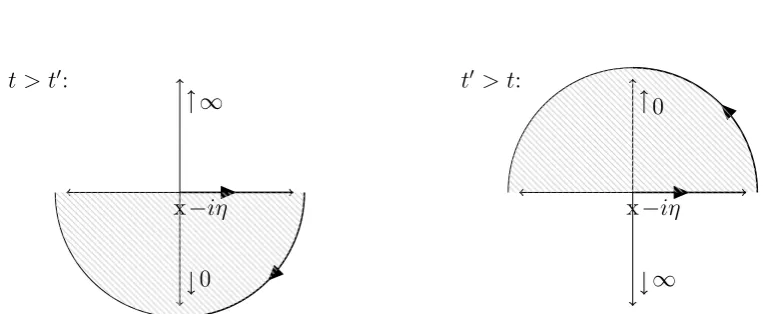
where η tends to zero, as can be seen from the residue theorem Z

Γ

f = 2πi X

a∈A(Γ)

where Γ is a closed counter-clockwise path in the complex plane that does not cross

itself and A(Γ) is the area enclosed by this path (cmp. Fig. 2.5). Similarly it is

straightforward to show that

Z ∞

−∞ 1 2πe

iκt _{dt=δ(κ) . (2.108)}

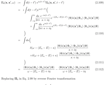
With Eqs. 2.105, 2.106, and 2.108 the Fourier transform of the polarization propa-gator is given by

Π0(x,x0, ω) :=

Z

d(t₋t0)eiω(t−t0)Π0(x,x0, t−t0) (2.109)

= i

Z

d(t₋t0)eiω(t−t0)

Z ∞

−∞

dκ

2πi

e−iκ(t−t0₎

κ+iη e

−i(En−E)(t−t0)_{hΦ|n˜(x)|Φ}

ni hΦn|n˜(x0)|Φi

+

Z ∞

−∞

dκ

2πi

eiκ(t−t0₎

κ+iηe

i(En−E)(t−t0)_hΦ|n˜(x0_)|Φ

ni hΦn|n˜(x)|Φi

(2.110)

= Z

dκ

δ(ω−(En−E)−κ) h

Φ|n˜(x)|Φni hΦn|n˜(x0)|Φi

κ+iη

+δ(ω+ (En−E) +κ) h

Φ|n˜(x0_)|Φ

ni hΦn|˜n(x)|Φi

κ+iη

(2.111)

= hΦ|n˜(x)|Φni hΦn|n˜(x 0_)|Φi

ω−(En−E) +iη −

hΦ|n˜(x0)|Φni hΦn|n˜(x)|Φi

ω+ (En−E)−iη

(2.112)

Replacing Π0 in Eq. 2.99 by reverse Fourier transformation

Π0(x,x0, t−t0) =

1 2π

Z

dω Π0(x,x0, ω)e−iω(t−t) (2.113)

the Fourier factors cancel

e−iω(t−t0)e−iω(t0−t00)_{· · ·}e−iω(t(n)−t) = 1 . (2.114)

Therefore the time-dependence of iΠ0 in the correlation energy (Eq. 2.99) can be

accounted for with a simple frequency integration.

EC =₋1 2

1 2π

Z

dω Tr_{log(1₋iΠ0(ω)Vee) +iΠ0(ω)Vee} (2.115)

2.4. RANDOM PHASE APPROXIMATION 25

H0 H

λ

t

0

Figure 2.4: The adiabatic connection is orthogonal to the adiabatic interaction of the Gell-Mann–Low theorem. The time-dependence of Hamiltonians in the interaction picture is de-picted here by fluctuations around the respective baselines. The non-interacting Hamiltonian is constant in time by construction and the full-interacting Hamiltonian is time-dependent throughout time, rendering solvation for its eigenstates difficult. Within the Gell-Mann–Low description the eigenstates are found for the non-interacting Hamiltonian and propagated due to a Hamiltonian that interpolates from the non-interacting to the interacting Hamilto-nian infinitely slowly, so that the fully interacting solution is found for t= 0. The adiabatic connection considers this process infinitely many times, following this process to various continuous degrees of physical interaction.

t > t0:

x₋iη ∞

0

t0 > t:

x₋iη

0

∞

2.4.5

Molecular Orbitals

Lehmann’s Representation in Molecular Orbitals

It yet remains to be shown how the transition values of the density fluctuation operator appearing in Eq. 2.112 can be evaluated in a molecular orbital basis. The sum over states _|Φnican be restricted to excited states by noting

hΦ_|n˜(x)_|Φni=hΦ|nˆ(x)−n(x)|Φi=

0 _| n= 0

hΦ|ˆn(x)|Φni | n6= 0 (2.116)

For excited states the transition density can be rewritten with the definition of the field operators (Eq. 2.35) as

hΦ_|nˆ(x)_|Φni=ϕ?p(x)ϕq(x)hΦ|ˆap†ˆaq|Φni . (2.117)

Unless|Φniis a singles excitation on|Φi(e.g. |Φaii), in which case Eq. 2.117 evaluates to 1, it vanishes exactly. For singles excitations the energy difference to the ground state is particularly simple to evaluate and Eq. 2.112 becomes

Π0(x,x0, ω) = ϕ?

i(x)ϕa(x)ϕa?(x0)ϕi(x0)

ω₋(εa−εi) +iη −

ϕ?

i(x0)ϕa(x0)ϕ?a(x)ϕi(x)

ω+ (εa−εi)−iη

. (2.118)

Real Molecular Orbitals

When all orbitals are real-valued (ϕp =ϕ?p), this allows for further simplification by a change of integration variable. As the numerators of both terms ofΠ0(ω) are equal in

this case, they can be factored out

iΠ0(x,x0, ω) =ϕi(x0)ϕa(x0)ϕa(x)ϕi(x) iPia(ω) (2.119)

with

Pia(ω) =

1

ω₋(εa−εi) +iη −

1

ω+ (εa−εi)−iη

. (2.120)

Pia(ω) vanishes for all of complex infinity, because

ω±(εa−εi)±iη |ω|→∞

−−−−→ω =|ω|eiφω _{. (2.121)}

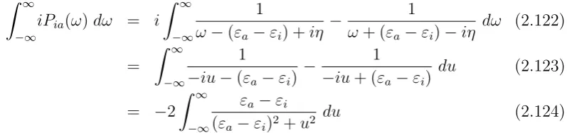
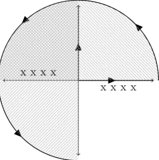
Therefore the integral over ω along the real axis in Eq. 2.115 can be closed over the upper half-plane. By comparison of the enclosed residues it becomes obvious that the integral from₋i_∞toi_∞closed over the left half-plane yields the identical result (cmp. Fig. 2.6).

Exchanging the integration variable for “imaginary frequency” u = iω therefore

results in

Z _∞

−∞

iPia(ω)dω = i

Z _∞

−∞

1

ω₋(εa−εi) +iη −

1

ω+ (εa−εi)−iη

dω (2.122)

=

Z ∞

−∞

1

−iu−(εa−εi) −

1

−iu+ (εa−εi)

du (2.123)

= −2

Z ∞

−∞

εa−εi (εa−εi)2+u2

2.4. RANDOM PHASE APPROXIMATION 27

x x

x x

x x

x x

Figure 2.6: The frequency integral over the polarization propagator in real Kohn–Sham orbitals can be carried out equivalently along the real axis or the imaginary axis. The contour can in both cases be closed in counter-clockwise direction and the only residues contained are those in the upper-left quadrant of the complex plane.

whereηhas been set identically to zero after the change of contour because it was only necessary to move the residues away from the integration (real) axis.

A regrouping of the terms, e.g.

Tr_{iΠ0(ω)Vee} = ϕi(x)ϕa(x)iPia(ω)ϕi(x0)ϕa(x0)Vee(x0,x) (2.125)

= iPia(ω)(ia|ia) (2.126)

and similarly

Tr_{iΠ0(ω)VeeiΠ0(ω)Vee} = iPia(ω)(ia|jb)iPjb(jb|ia) (2.127)

delivers the final formulation of the correlation energy in real molecular orbitals

EC =₋ Z _du

4π Tr{log(1 +Q(u)V)−Q(u)V} (2.128)

with

Qia,jb(ω) = 2

εa−εi (εa−εi)2 +u2

δia,jb (2.129)

Chapter 3

Publications

In this chapter, the original research of the present work will be presented. It was first published in peer-reviewed journals and is reprinted on the following pages in the original format. The supporting materials that have been published together with the manuscripts are also reproduced for completeness.

3.1

AO-RI-RPA

H. F. Schurkus and C. Ochsenfeld,

J. Chem. Phys. (Communication) 144, 031101 (2016)

An effective linear-scaling atomic-orbital reformulation of the random-phase approximation using a contracted double-Laplace transformation

Abstract from the publication: An atomic orbital (AO) reformulation of the

random-phase approximation (RPA) correlation energy is presented allowing to reduce the steep computational scaling to linear, so that large systems can be studied on simple desktop computers with fully numerically controlled accuracy. Our AO-RPA formula-tion introduces a conctracted double-Laplace transform and employs the overlap-metric resolution-of-the-identity. First timings of our pilot code illustrate the reduced scaling with systems comprising up to 1262 atoms and 10 090 basis functions.

The following article is reproduced in agreement with its publisher (AIP Publishing LLC) and can be found online at

3.1. AO-RI-RPA 31

THE JOURNAL OF CHEMICAL PHYSICS144, 031101 (2016)

Communication: An effective linear-scaling atomic-orbital reformulation

of the random-phase approximation using a contracted double-Laplace

transformation

Henry F. Schurkus and Christian Ochsenfeld

Chair of Theoretical Chemistry and Center for Integrated Protein Science Munich (CIPSM), Department of Chemistry, University of Munich (LMU), D-81377 Munich, Germany

(Received 2 December 2015; accepted 30 December 2015; published online 20 January 2016)

An atomic-orbital (AO) reformulation of the random-phase approximation (RPA) correlation energy is presented allowing to reduce the steep computational scaling to linear, so that large systems can be studied on simple desktop computers with fully numerically controlled accuracy. Our AO-RPA formulation introduces a contracted double-Laplace transform and employs the overlap-metric resolution-of-the-identity. First timings of our pilot code illustrate the reduced scaling with systems comprising up to 1262 atoms and 10 090 basis functions. C 2016 AIP Publishing LLC.[http://dx.doi.org/10.1063/1.4939841]

I. INTRODUCTION

The random phase approximation (RPA) originally introduced by Bohm and Pines1_{has become of wide interest} for describing electron-correlation both in solid-state and molecular systems offering important advantages also for vanishing electronic gap systems. However, the applicability of RPA to larger systems has always suffered from its huge computational cost. For molecular systems the currently most widespread RPA formulation employing the resolution-of-the-identity (RI) approximation was proposed by Furcheet al.,2–4 on the basis of formulations by Langreth and Perdew,5,6_and reduces the effective scaling from O M6 _{to O M}4 _with

system size M. This opened the way for more extensive benchmarking beyond the few atoms scale. Many authors have consequently shown the usefulness and applicability of RPA.7–12 _{Developments include analytical forces and} first-order properties by Rekkedal et al.13 _{and Burow et al.,}14 the stochastic reformulation by Gaoet al.,15_{and a complete} basis set extrapolation by Mezeiet al.16 _{Recently, Kállay}17 presented an effective linear-scaling approximation using a local correlation domain-based approach. While not all of the employed approximations for preselecting domains are rigorous, Kállay presented for the tightest selection criteria deviations in relative energies on the order of 1 kcal/mol for a range of selected molecular systems. However, further increasing the accuracy, full rigorosity, and, e.g., avoiding domain changes on a potential energy surface remain difficult. In our work, we present an effective linear-scaling RPA atomic orbital (AO) reformulation entirely avoiding ad-hoc approximations in order to recover the exact RPA results and allows for full numerical control of the accuracy by simple thresholding in the spirit of direct SCF or other rigorous AO-based methods. This opens up the possibility to study molecules of several hundreds to thousands of atoms at the RPA level on a simple desktop computer, while the accuracy remains fully numerically controlled.

Our formulation employs a contracted double-Laplace transformation and a RI-expansion in the overlap-metric

formulation. While the Coulomb-metric formulation is far more common than the overlap-metric nowadays, the three-center overlap allows us directly to reformulate all time-limiting steps in sparse quantities allowing for linear scaling sparse matrix algebra. In contrast to the widespread expectation that the overlap-metric would entail the need for very large auxiliary basis sets, we do find errors much smaller than the intrinsic error of RPA already for standard auxiliary basis sets (e.g., cc-pVQZ-RI for the cc-pVQZ basis18–22_).

Yang and co-workers23 _{have previously suggested to} use tensor hypercontraction (THC) methods instead of the RI-expansion for rank reduction within RPA. THC allows to express the electron repulsion integrals solely by rank-2 tensors, while the overlap metric RI also includes rank-3 tensors. The highest rank tensors in RI are, on the other hand, limited to linear increase of significant elements with molecular size, which is a necessity of our linear scaling reformulation. In the context of periodic systems computed with plane wave basis sets, Kresse and co-workers24 _have recently used the simple Laplace integration together with a Fourier transformation scheme to reduce the scaling to cubic, finding that the grids originally developed for second-order Møller-Plesset (MP2) theory are also suited for use with RPA. This goes well with our finding that also for our new contracted double-Laplace scheme the original MP2 grids already perform sufficiently well.

In the following, first the derivation of our RPA reformulation is given, including a discussion on numerical stability. Then the efficiency and scaling behavior of our pilot implementation are described. Finally, a brief outlook on possible further improvements is presented.

II. THEORY

RPA has been found to be a highly useful correlation method for going beyond approximative forms of Kohn-Sham density-functional theory (KS-DFT).2,7–12_{Here, RPA is} generally derived from the adiabatic connection25_{as presented}