Scale effects in quasi-fragile materials subjected to compression

(1)

SCALE EFFECTS IN QUASI-FRAGILE MATERIALS SUBJECTED TO

COMPRESSION

I. Iturrioz1, J.D. Riera2, L.F.F. Miguel1, L.E. Kosteski1

1_{Department of Mechanical Engineering, UFRGS, Porto Alegre, Brazil} 2_{Department of Civil Engineering, UFRGS, Porto Alegre, Brazil} E-mail of corresponding author: ignacio@mecanica.ufrgs.br

ABSTRACT

In the truss-like Discrete Element Method (DEM), masses are considered lumped at nodal points and interconnected by means of unidimensional elements with arbitrary constitutive relations. In previous studies of the tensile fracture behavior of concrete cubic samples, it was verified that numerical predictions of fracture of non-homogeneous materials using DEM models are feasible and yield results that are consistent with the experimental evidence so far available. Applications that demand the use of large elements, in which extensive cracking within the elements of the model may be expected, require the consideration of the increase with size of the fractured area, in addition to the effective stress-strain curve for the element. This is a basic requirement in order to achieve mesh objectivity. Note that the degree of damage localization must be known a priori, which is a still unresolved difficulty of the non-linear fracture analysis of non-homogeneous large structures. Results of the numerical fracture analysis of 2D systems employing the DEM were also reported by the authors and compared with predictions based on the multi-fractal theory proposed by Carpinteri et al. according to which a fractal dimension ∆, contained in the interval (1-2), defines the fracture area for a unitary thickness. The influence of various parameters, such as the mesh size, the strain velocity and the shape of the fracture surface were thus assessed by means of numerical simulation in samples subjected to tensile stresses. Elements subjected to compression actually fail by indirect tension. Such cases - the standard test to determine the so-called compressive strength of concrete is an important example - are more difficult to simulate or to relate to the fractal theory advanced by Carpinteri et al., partly because the peak load is reached before sliding with friction occurs along failure surfaces. This paper presents preliminary results of prismatic concrete samples subjected to static compression obtained by simulation with the Discrete Element Method. The results include simulations with and without friction at the end platens leading to reliable prediction of the sample behavior up to the peak load.

INTRODUCTION

It is quite clear now that for predicting the response up to failure of solids subjected to dynamic loads, in particular post-peak response, methods based on Continuum Mechanics present disadvantages in comparison with discrete models of the solids under consideration. This is a consequence of material fracture, which introduces discontinuities in the displacement functions that are difficult to handle in a continuum formulation and fostered the rapid development of more efficient and natural methods of analysis. Among various such alternative methods, the so-called truss-like Discrete Element Method proved quite useful. The approach was proposed by Riera [1] to determine the dynamic response of plates and shells under impact loading when failure occurs primarily by shear or tension, which is generally the case in concrete structures. The lack of sufficient experimental evidence in this area to confirm structural responses determined with the method, led to the assessment of its predicting capability in structures subjected to quasi-static loading.

(2)

if the appropriate stress-strain relations are adopted. These relations depend both on the size of the element and on the correlation lengths of the random fields that describe the relevant material properties.

In response determinations of structures with initial cracks or high stress gradients, which result in fracture localization, well established procedures lead to results that are mesh independent. However, in elements subjected to approximately uniform stress fields a hitherto unknown problem arises in the analysis of non-homogeneous materials: the need to know a priori the degree of fracturing of the element. This also affects finite element analysis in cases in which there is no clear fracture localization, requiring a careful evaluation of the energy dissipated by fracture or other mechanisms in the course of the loading process. Tentative criteria to account for the effect in non-linear dynamic fracture analysis of large structural systems were proposed by Riera et al. [7].

Elements subjected to compression actually fail by indirect tension. Such cases - the standard test to determine the so-called compressive strength of concrete is an important example - are more difficult to simulate or to relate to the fractal theory advanced by Carpinteri et al. [8], partly because the peak load is reached before sliding with friction occurs along failure surfaces. This paper presents preliminary results of prismatic concrete samples subjected to static compression obtained by simulation with the Discrete Element Method. The results include simulations with and without friction at the end platens, leading to close prediction of the sample behavior, including the cracking pattern, up to the peak load. Research is presently under way to extend the predicting capability of the method to the post-peak behavior in elements subjected to compressive loads.

THE DISCRETE ELEMENT METHOD IN FRACTURE PROBLEMS

The Discrete Element Method employed in this paper is based on the representation of a solid by means of an arrangement of elements able to carry only axial loads The discrete elements representation of the orthotropic continuum was adopted to solve structural dynamics problems by means of explicit direct numerical integration of the equations of motion, assuming the mass lumped at the nodes. Each node has three degrees of freedom, corresponding to the nodal displacements in the three orthogonal coordinate directions. The equations that relate the properties of the elements to the elastic constants of an isotropic medium are:

9 4 8

ν δ

ν =

− ,

(

)

2 9 8

2 9 12

n

EA EL δ

δ + =

+ ,

2 3 3

d n

EA = A (1)

in which E and ν denote Young’s modulus and Poisson’s ratio, respectively, while An and Ad represent the areas of normal and diagonal elements. The resulting equations of motion may be written in the well-known form:

( ) ( )

0

r

x+ x+F t −P t =

M C

r r r r

&& & (2)

in which xr represents the vector of generalized nodal displacements, M the diagonal mass matrix, C the damping

matrix, also assumed diagonal, F t_r

( )

r

the vector of internal forces acting on the nodal masses and P t

( )

r

the vector

of external forces. Obviously, if M and C are diagonal, Eq. (2) are not coupled. Then the explicit central finite

differences scheme may be used to integrate Eq. (2) in the time domain. Since the nodal coordinates are updated at every time step, large displacements can be accounted for in a natural and efficient manner. In the present paper, the relation between tensile stress and strain in the material was assumed to be triangular, as shown in Fig.1. Another important feature of the approach is the assumption that Gf is not constant throughout the structure. In this paper, following previous contributions, it is assumed that Gf has a Weibull distribution. It should be underlined again that fracture localization weakens as the non-homogeneous nature of the material becomes more pronounced, i.e., as the coefficients of variation of the variables that describe the material properties increase. Applications of the DEM in studies involving non-homogeneous materials subjected to fracture, like concrete and rock, may be found in [5,9,10].

NON-LINEAR CONSTITUTIVE MODEL FOR MATERIAL DAMAGE

(3)

Thus, for a given point P on the force vs. strain curve, the area of the triangle OPC represents the reversible elastic energy density stored in the element, while the area of the triangle OAP is proportional to the energy density dissipated by damage. Once the damage energy density equals the fracture energy, the element fails and loses its load carrying capacity. On the other hand, in the case of compressive loads the material behavior is assumed linearly elastic. Thus, failure in compression is induced by indirect tension.

Fig.1: Triangular constitutive law adopted for DEM uni-axial elements.

Constitutive parameters and symbols are shown in Figure 1 [11]. The element axial force F depends on the axial strain ε. The area associated to each element is given by Eq. (6) for longitudinal and diagonal elements. An equivalent fracture area Ai* of each element is defined in order to satisfy the condition that the energies dissipated by fracture of the continuum and by its discrete representation are equivalent. With this purpose, fracture of a cubic sample of dimensions L×L×L is considered. The energy dissipated by fracture of a continuum cube due to a crack parallel to one of its faces is:

2

f f

G G L

Γ = Λ = (3)

which Λ is the actual fractured area, i.e., L2. On the other hand, the energy dissipated when a DEM module of dimensions L×L×L fractures in two parts consists of the contributions of five longitudinal elements (four coincident with the module edges and an internal one) and four diagonal elements.

Then, the energy dissipated by the DEM module can be written as follows [12]:

2 2 DEM

2

4 0.25 4

3

f A A A

G c c c L

 _ _ 

 

Γ = _ + +   _

 

(4)

The first term between brackets accounts for the four edge elements, the second term for the internal longitudinal element, while the third term represents the contribution of the four diagonal elements. The coefficient cA is a scaling parameter used to establish the equivalence between Γ and ΓDEM. Thus:

2 22 2

3

f f A

G L =G _ c _L

  (5)

from which it follows that cA = 3/22. Finally, the equivalent fracture areas of longitudinal and diagonal elements are:

Al* = (3/22) L2, Ad* = (4/22) L2 (6) Damage energy,

Udmg

Elastic strain energy, Uel EAi

F

ε εp

P

O

A

C

B

(4)

These values apply as long as there is a single large crack in the element. The critical failure strain (εp) is defined as the largest strain attained by the element before the damage initiation (point A in Figure 1). The relationship between εp and the specific fracture energy Gf is given in terms of Linear Elastic Fracture Mechanics as:

(

2

)

1

f

p f

G

R

E

ε

ν

=

−

(7)

in which Rf is the so-called failure factor, which may accounts for the presence of an intrinsic defect of size a. Rf may be expressed in terms of a as:

1

f

R

Y a

=

(8)

in which Y is a dimensionless parameter that depends on both the specimen and crack geometry. The element loses its load carrying capacity when the limit strain εr is reached (Point B in Figure 1). This value must satisfy the condition that, upon failure of the element, the dissipated energy density equals the product of the element fracture area Ai* times the specific fracture energy Gf, divided by the element length. Hence:

( )

* 2

0 2

r

f i r p i

i

G A K E A

F d

L

ε

ε ε= =

∫

(9)

in which the sub index i is replaced by l or d depending on whether the element under consideration is a longitudinal or diagonal. The coefficient Kr is a function of the material properties and the element length Li:

*

2

f i

r

i i

p

G A

K

A L

Eε

   

=_ _  

   

 

(10)

In order to guarantee the stability of the algorithm, the condition Kr≥ 1 must be satisfied. In this sense it is interesting to define the critical element length:

*

2

2 f i

cr

i p

G A

L

A Eε

   

= _   

  

  (11)

(Al*/ Al) = (3/22) / φ, (Ad*/ Ad) = ( 3 11)/ (δφ) (12)

In the special case of an isotropic continuum with ν = 0.25, the value of the coefficients above are δ = 1.125 and φ = 0.4, which leads to (Al*/ Al) ≈ (Ad*/ Ad) ≈ 0.34. Thus, for practical purposes, a single value of the critical length can be used for longitudinal and diagonal elements. Therefore, the stability condition may be expressed as:

1

cr

r i cr

i

L

K L L

L

= ≥ ⇒ _≤ (13)

Finally, the expression for the limit strain is:

r

ε

=Krεp. (14)

(5)

The random distribution of material parameters in the DEM environment

Miguel et al. [5,13] and Iturrioz et al. [14] modeled the random properties of material assuming the toughness Gf as a random field with a Type III (Weibull) extreme value distribution, given by Eq. (15):

( )

_f 1 exp

(

_f

)

F G = − _− G β γ_

  (15)

in which β and γ are the scale and shape parameters, respectively. The mean value (µ) and the standard deviation (s) of Gf are given by:

(

1 1

)

µ β= _Γ + γ _ (16)

(

)

₂

(

)

1 2

1 2 1 1

s=β_Γ + γ − Γ + γ _ (17)

in which

( )

1

0

x t

x ∞ − −t e dt

Γ =

_∫

denotes the Gamma function. In order to simulate pseudo random values of Gf the

following expression was used:

(

)

1 ln 1 f

G =β_− −u _ γ (18)

in which u is a random number with uniform probability distribution in the interval (0,1). Routines for generating samples of u are widely available. In earlier applications of the DEM, by taking the size of the elements (L) equal to the correlation length of the random field of the material property of interest, say lc, allowed assuming that simulated values were uncorrelated, thus simplifying the computational scheme. This is however an important limitation of the model, initially addressed by Rios [2]. Later, Miguel [15] adopted the method proposed by Shinozuka and Deodatis [16] to simulate a gaussian 3D random field to model the material property of interest. A simpler technique was employed by Puglia et al. [17]. This method was used herein to simulate the 3D random field that describes the toughness Gf, which is then independent of the discretization adopted in the DEM.

Thus, in the following analysis a DEM mesh is generated. Then, random values of the desired property are generated, according to the specified probability distribution function, at nodal points in a 3D grid with lengths (lcx, lcy, lcz) in the three Cartesian directions. lcx, lcy and lcz represent the correlation lengths of the random field in the x,y,z directions. The random values at the location of DEM elements are determined by a linear 3D interpolation from the values at the nodes. Additional details may be found in [17].

ANALYSIS OF PRISMATIC SAMPLES SUBJECTED TO COMPRESSION

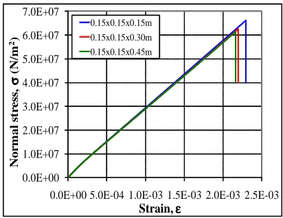
Concrete prismatic samples fixed at the lower face and subjected to a monotonically increasing uniformly distributed compression displacement on the upper face were analyzed. The response of each sample up to failure was determined through numerical simulation. Two sets with different boundary conditions were analyzed. First, in Case A, the samples were analyzed with restrictions in x and y directions on the nodes on the upper and lower faces. Next, in Case B, the same samples were analyzed without restrictions in both x and y directions. Samples with 0.15×0.15m cross sectional area and 0.15, 0.30 and 0.45m lengths were analyzed. The size L of DEM elements was 0.015m in all cases. Hence, the three sample sizes contain 10×10×10; 10×10×20 and 10×10×30 modules, respectively. The material properties of concrete are: Young’s modulus, E = 3.5E10N/m2; mass density, ρ = 2400kg/m3 and Poisson’s ratio, ν= 0.25. In the ensuing simulations, only the specific fracture energy, Gf was modeled as a random field, with mean 90N/m and a coefficient of variation equal to 2. The critical strain εp was assumed equal to 3.9E-5.

(6)

simulations is also shown in Figs. 2 and 3, while the mean curves for the three sizes are shown for Case B in Fig. 4. Note that for the cubic specimen the stress-strain curve is approximately linear up to the peak value, while for the prismatic specimens inflexion points are visible at a normal stress of around 1.0E+07, indicating the initiation of damage by indirect tension.

(a) (b) (c)

Fig. 2: Normal stress on the lower face vs. mean strain for all simulations and resulting mean curve (thick black line), (a) 0.15×0.15×0.15m cube, (b) 0.15×0.15×0.30m prism and (c) 0.15×0.15×0.45m prism, for Case A.

(a) (b) (c)

Fig. 3: Normal stress on the lower face vs. mean strain for all simulations and resulting mean curve (thick black line), (a) 0.15×0.15×0.15m cube, (b) 0.15×0.15×0.30m prism and (c) 0.15×0.15×0.45m prism, for Case B.

0.0E+00 1.0E+07 2.0E+07 3.0E+07 4.0E+07 5.0E+07 6.0E+07 7.0E+07

0.0E+00 5.0E-04 1.0E-03 1.5E-03 2.0E-03 2.5E-03

N o r m a l st r e ss , σσσσ (N /m 2)

Strain, εεεε

0.15x0.15x0.15m 0.15x0.15x0.30m 0.15x0.15x0.45m

Fig. 4: Normal stress on the lower face vs. mean strain for the mean curve of the three sample sizes, for Case B (without restrictions in x and y directions).

-1.0E+07 0.0E+00 1.0E+07 2.0E+07 3.0E+07 4.0E+07 5.0E+07 6.0E+07 7.0E+07 8.0E+07

0.0E+00 1.0E-03 2.0E-03 3.0E-03

N o rm a l st re ss , σσσσ (N /m 2)

Sim 1 Sim 2 Sim 3 Sim 4 Sim 5 Sim 6 Mean -1.0E+07 0.0E+00 1.0E+07 2.0E+07 3.0E+07 4.0E+07 5.0E+07 6.0E+07 7.0E+07 8.0E+07

0.0E+00 1.0E-03 2.0E-03 3.0E-03

Sim 1 Sim 2 Sim 3 Sim 4 Sim 5 Sim 6 Mean -1.0E+07 0.0E+00 1.0E+07 2.0E+07 3.0E+07 4.0E+07 5.0E+07 6.0E+07 7.0E+07 8.0E+07

0.0E+00 1.0E-03 2.0E-03 3.0E-03

Sim 1 Sim 2 Sim 3 Sim 4 Sim 5 Sim 6 Mean -1.0E+07 0.0E+00 1.0E+07 2.0E+07 3.0E+07 4.0E+07 5.0E+07 6.0E+07 7.0E+07

0.0E+00 1.0E-03 2.0E-03 3.0E-03

(7)

Fig. 5: Rupture configuration of concrete samples subjected to compression (controlled displacements on upper face). Note that only damage at central slices of the samples is shown.

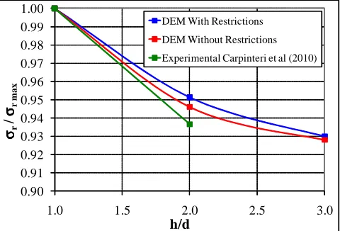
Typical crack patterns are shown in Figure 5. Unbroken elements are represented in black while broken elements were deleted for clarity. The graphs show both a typical fracture pattern, as well as the damage distribution in the sample. Figure 6 shows a comparison of DEM results, with and without restrictions to lateral motions at the end platens, with experimental values obtained by Carpinteri et al. [18]. It is important to note that the value CV = 2 adopted in the analysis for the specific fracture energy of concrete unidimensional DEM elements Gf, results in CVs of around 0.09 for the rupture stress σrup and for the rupture strain εrup, for the 0.15m cube with restrictions to lateral motion in x and y directions on the upper and lower faces (Case A). The authors are not aware of any direct experimental assessment of CV(Gf), but regard both CV(σrup) and CV(εrup) compatible with experimental evidence.

0.90 0.91 0.92 0.93 0.94 0.95 0.96 0.97 0.98 0.99 1.00

1.0 1.5 2.0 2.5 3.0

σσσσr

/

σσσσr m

a

x

h/d

DEM With Restrictions

DEM Without Restrictions

Experimental Carpinteri et al (2010)

Fig. 6: Comparison between present numerical and Carpinteri et al. [18] experimental results.

CONCLUSIONS

Continuing previous applications of the Discrete Element Method (DEM) to the fracture analysis of non-homogeneous quasi fragile materials, the authors presented in the paper preliminary results of the response of cubic and prismatic concrete samples subjected to static compression, obtained by numerical simulation. The results include simulations with and without friction at the end platens, leading to robust predictions of the sample behavior up to the peak load. Comparison with available experimental results suggest that size effects as well as strain rate

15x15x15m 15x15x15m

15x15x30m 15x15x30m

15x15x45m 15x15x45m

(8)

effects –not reported in this paper– are correctly accounted for by the model. Finally, while in the analysis of samples subjected to tension and/or shear at constant strain rates the entire load-displacement curve is satisfactorily predicted, in compression this is not the case and additional research is needed to avoid the sudden rupture predicted by the present model.

Acknowledgements. The authors acknowledge the support of CNPq and CAPES (Brazil).

REFERENCES

[1] Riera, J.D., “Local effects in impact problems on concrete structures”. Proceedings, Conference on Structural Analysis and Design of Nuclear Power Plants. Oct. 1984, Porto Alegre, RS, Brasil, Vol. 3, CDU 264.04:621.311.2:621.039.

[2] Rios, R.D, Riera, J.D., “Size effects in the analysis of reinforced concrete structures”, Engineering Structures, Elsevier, Vol. 26, pp. 1115-1125, 2004.

[3] Hillerborg, A., “A model for fracture analysis”, Cod. LUTVDG/TVBM 300-51-8, 1971.

[4] Van Vliet, M.R.A, Van Mier, J.G.M, “Size effects of concrete and sandstone”, Heron, Vol 45, No.2, pp. 91-108, 2000.

[5] Miguel, L.F.F., Riera, J.D., Iturrioz, I., “Influence of size on the constitutive equations of concrete or rock dowels”, Int J Numer Anal Meth Geomech, Vol. 32, No. 15, pp. 1857-188, 2008. DOI: 10.1002/nag.699. [6] Riera, J.D., Iturrioz, I., “Size effects in the analysis of concrete or rock structures”, International

Conference on Structural Mechanics in Reactor Technology (SMiRT 19), Toronto, Canada, 2007.

[7] Riera, J.D., Iturrioz, I., Miguel, L.F.F., “On Mesh Independence in Dynamic Fracture Analysis by Means of the Discrete Element Method”. ENIEF 2008 - XVII Congreso sobre Métodos Numéricos y sus Aplicaciones, San Luis, Argentina, Vol. XXVII, pp. 2085-2097, 2008.

[8] Carpinteri, A., Chiaia, B., “Multifractal Scaling laws in the breaking Behaviour of Disordered Materials”, Chaos Solitons & Fractals, Vol, 8, No. 2, pp. 135-150, 1997.

[9] Riera, J.D., Iturrioz, I. “Discrete elements model for evaluating impact and impulsive response of reinforced concrete plates and shells subjected to impulsive loading”. Nuclear Engineering and Design, Vol. 179, pp. 135-144, 1998.

[10] Dalguer, L.A., Irikura, K., Riera, J.D., Chiu H.C., “The importance of the dynamic source effects on strong ground motion during the 1999 Chi-Chi, Taiwan, earthquake: Brief interpretation of the damage distribution on buildings”. Bull. Seismol. Soc. Am., Vol. 91, pp. 1112-1127, 2001.

[11] Rocha, M.M., Riera, J.D., Krutzik N.J., “Extension of a model that aptly describes fracture of plain concrete to the impact analysis of reinforced concrete”, Int. Conf. and Structural Mechanics in Reactor Technology, SMiRT 11, Trans. Vol. J., Tokyo, Japan. 1991.

[12] Kosteski, L.E., Riera, J.D., Iturrioz, I., “Consideration of Scale Effects and Stress Localization in Response Determination Using the DEM”, MECOM – CILAMCE 2010, November 2010, Buenos Aires, Argentina. Mecánica Computacional, Vol XXIX, pp. 2785-2801, 2010.

[13] Miguel, L.F.F., Iturrioz, I., Riera, J.D., “Size Effects and Mesh Independence in Dynamic Fracture Analysis of Brittle Materials”, Computer Modeling in Engineering & Sciences, Vol. 56, pp. 1-16, 2010. [14] Iturrioz, I., Miguel, L.F.F., Riera, J.D., “Dynamic Fracture Analysis of Concrete or Rock Plates by Means

of the Discrete Element Method”, LAJSS, Vol. 6, pp. 229-245, 2009.

[15] Miguel, L.F.F., “Critério constitutivo para o deslizamento com atrito ao longo da falha sísmica”, Ph.D. thesis, PPGEC, Escola de Engenharia, UFRGS, Porto Alegre, Brazil, 2005.

[16] Shinozuka M., Deodatis G., “Simulation of Multidimensional Gaussian Stochastic Fields by Spectral Representation”, Apl. Mech. Rev, Vol. 49, no 1, January 1996.

[17] Puglia, B.V., Iturrioz, I, Riera, J.D., Kosteski, L., “Random field generation of the material properties in the truss-like discrete element method”, Mecánica Computacional, Cilamce-Mecom 2010, Vol. XXIX, pp. 6793-6807, 2010.