SIMPLIFIED SSI MODEL FOR FLEXIBLE SHALLOW OR EMBEDDED
FOUNDATIONS
Alberto Frau1, Fan Wang2
1Research Engineer, CEA, DEN, DANS, DM2S, SEMT, Laboratoire d’Etudes de Mécanique Sismique.
F-91191 Gif-sur-Yvette. ([email protected])
2Research Engineer, CEA, DEN, DANS, DM2S, SEMT, Laboratoire d’Etudes de Mécanique Sismique.
F-91191 Gif-sur-Yvette.
ABSTRACT
In conducting seismic risk assessment during the early design stage of buildings, several phenomena could be very difficult to be taken into account. For example, Soil Structure Interactions (SSI) could be modelled with several methods (“full FEM” or “FEM-BEM”). But these approaches could be very expensive in terms of computational time, so they are not always available for a design study. For this reason, simplified approaches are often employed in which a rigid soil-structure interface is assumed. Nevertheless in some cases, this condition could not be used, especially for structures with flexible embedded foundations, thus other approaches must be used in order to avoid this limitation.
In this paper, a new method is proposed in order to model the SSI effect for a flexible foundation (shallow or embedded). For the embedded configuration, the evaluation of the Foundation Input Motion (FIM) is also necessary. A simplified approach is proposed to determinate the kinematic interaction with the foundation.
Numerical tests (a reactor building coupled with a multi-layered soil under seismic loading) conducted for our model showed its capacity to represent the behaviour of the soil-structure system under earthquake loadings for a given frequency range.
INTRODUCTION
For the resolution of Soil Structure Interaction (SSI) problems, several types of methods exist. Two of these are the “full FEM” and “FEM-BEM” methods. Generally, these methods are able to represent very well all kinds of phenomena behind the SSI problems. But these approaches are very expensive in terms of computational time. For this reason, the SSI effects are not considered in certain situations especially in the early design stage.
In the literature, several works exist concerning the simplification of the SSI approach. One of the best known is the method described by Wolf (1988). This is formulated in order to represent the dynamic stiffness (especially the frequency dependence of the impedances functions) of a rigid soil-structure interface founded on a homogenous soil. Still on this subject, another kind of models used for the rigid interface is the macro-element models (Cremer and al (2001)) that are formulated to model the nonlinear behaviour in the static case. An extension to the dynamic problems was proposed by Grange (2009). But in the first version the frequency dependence was not considered.
difficult in certain cases. In the first part of this article, we propose a simplified model, based on Wolf’s (1988) approach and defined in a heuristic way.
Another aspect concerning the simplified SSI models is the definition of the Foundation Input Motion (FIM) in the embedded configuration. Supposing that we have a free field signal as input data, the kinematic interaction between the soil and the massless structure and the reduction of the free field signal as a function of depth, impact directly the FIM. Several studies have been published concerning this problem (Kausel and al. (1978), Kurimoto and al. (1996)) and they are based on the rigid interface hypothesis (classical hypothesis for the Sway-Rocking model). But for deep embedded foundations, this condition is not always satisfied. Thus, in the second part of this article, we have carried out an extension of the Kausel’s work to flexible foundations. Finally, a numerical case has been studied to test the two proposed approaches.
SIMPLIFIED SSI MODEL
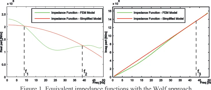
Regarding the Wolf (1988) approach, using the impedances functions of a massless rigid foundation, it is possible to define an equivalent lumped mass system composed of three terms: springs, mass and dashpot, for each DoF.
Figure 1. Equivalent impedance functions with the Wolf approach.
These values can be obtained with respect to three frequencies݂ଵ, ݂ଶ and ݂ଷ.
݇ிൌ Ըሾܫ݉ிሺ݂ଵሻሿ (1)
݉ி ൌ ሺԸሾܫ݉ிሺ݂ଵሻሿ െ Ըሾܫ݉ிሺ݂ଶሻሿሻȀሺʹߨ݂ଶሻଶ (2)
ܿிൌ Աሾܫ݉ிሺ݂ଷሻሿȀሺʹߨ݂ଷሻ (3)
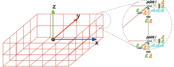
Figure 2. Distribution of the stiffness, mass and damping terms.
The distribution is carried out in the following way:
൞
݇௫ ൌ ݇௫ሺሻ ݇ȁݔȁ
݇௬ ൌ ݇௬ሺሻ ݇ȁݕȁ
݇௭ ൌ ݇௭ሺሻ ݇ሺଵሻ௭ ȁݔȁ ݇௭ሺଶሻȁݕȁ
(4)
൞
݉௫ ൌ ݉௫ሺሻ ݉ȁݔȁ
݉௬ ൌ ݉௬ሺሻ ݉ȁݕȁ
݉௭ ൌ ݉௭ሺሻ ݉௭ሺଵሻȁݔȁ ݉௭ሺଶሻȁݕȁ
(5)
൞
ܿ௫ ൌ ܿ௫ሺሻ ܿȁݔȁ
ܿ௬ ൌ ܿ௬ሺሻ ܿȁݕȁ
ܿ௭ൌ ܿ௭ሺሻ ܿ௭ሺଵሻȁݔȁ ܿ௭ሺଶሻȁݕȁ
(6)
Consequently, the problem is to determine the 18 parametersቄ݇௫ሺሻǡ ݇௬ሺሻǡ ݇ǡ ݇௭ሺሻǡ ݇௭ሺଵሻǡ ݇௭ሺଶሻቅ; ቄ݉௫ሺሻǡ ݉௬ሺሻǡ ݉ǡ ݉௭ሺሻǡ ݉௭ሺଵሻǡ ݉௭ሺଶሻቅ and ቄܿ௫ሺሻǡ ܿ௬ሺሻǡ ܿǡ ܿ௭ሺሻǡ ܿ௭ሺଵሻǡ ܿ௭ሺଶሻቅ in equations (4), (5) and (6). Using
the 18 values defined by the equations (1), (2) and (3) (3 for each DoF), a set of equations could be defined.
It is possible to link the local values of stiffness, damping and mass for each interface point (ൣ݂݇݀݅ ǡ ݂݉݀݅ ǡ ݂ܿ݀݅ ൧ǡ ݂݀ ൌ ݔǡ ݕǡ ݖ) to their global values using the follow relations:
ቐ
݇௫௫ ൌ ܨ௫Ȁݑ௫ൌ ሺσேୀଵ݇௫ݑ௫ሻȀݑ௫
݇௬௬ൌ ܨ௬Ȁݑ௬ൌ ൫σேୀଵ݇௬ݑ௬൯Ȁݑ௬
݇௭௭ ൌ ܨ௭Ȁݑ௭ൌ ሺσேୀଵ݇௭ݑ௭ሻȀݑ௭
൞
݇ఏ௫ൌ ܯ௫Ȁߠ௫ൌ ൫σேୀଵ݇௭ݑ௭ݕെ ݇௬ݑ௬ݖ൯Ȁߠ௫
݇ఏ௬ൌ ܯ௬Ȁߠ௬ൌ ሺσேୀଵ݇௫ݑ௫ݖെ ݇௭ݑ௭ݔሻȀߠ௬
݇ఏ௭ൌ ܯ௭Ȁߠ௭ൌ ൫σேୀଵ݇௬ݑ௬ݖെ ݇௭ݑ௭ݔ൯Ȁߠ௭
(7)
൞
ܿ௫௫ ൌ ܥ௫Ȁݑ௫ሶ ൌ ሺσ ܿேୀଵ ௫ݑప௫ሶሻȀݑ௫ሶ
ܿ௬௬ ൌ ܥ௬Ȁݑ௬ሶ ൌ ሺσ ܿேୀଵ ௫ݑప௫ሶ ሻȀݑ௬ሶ
ܿ௭௭ ൌ ܥ௭Ȁݑ௭ሶ ൌ ሺσ ܿேୀଵ ௫ݑప௫ሶ ሻȀݑ௭ሶ
൞
ܿఏ௫ൌ ܯఏ௫Ȁߠ௫ሶ ൌ ൫σ ܿேୀଵ ௭ݑ௭పሶ ݕെ ܿ௬ݑ௬పሶ ݖ൯Ȁߠ௫ሶ
ܿఏ௬ൌ ܯఏ௬Ȁߠ௬ሶ ൌ ሺσ ܿேୀଵ ௫ݑ௫పሶ ݖെ ܿ௭ݑ௭పሶ ݔሻȀߠ௬ሶ
ܿఏ௭ൌ ܯఏ௭Ȁߠሶ ൌ ൫σ ܿ௭ ேୀଵ ௬ݑ௬పሶ ݖെ ܿ௭ݑ௭పሶ ݔ൯Ȁߠ௭ሶ
(8)
൞
݉௫௫ൌ ሺσேୀଵ݉௫ሻ
݉௬௬ൌ ൫σேୀଵ݉௬൯
݉௭௭ൌ ൫σேୀଵ݉௬൯
൞
݉ఏ௫ ൌ ሺσேୀଵ݉௭ݕଶ ݉௫ݖଶሻ
݉ఏ௫ൌ ൫σேୀଵ݉௭ݔଶ ݉௬ݖଶ൯
݉ఏ௫ ൌ ൫σேୀଵ݉௬ݔଶ ݉௫ݕଶ൯
(9)
terms ൛ݑ௫ǡ ݑ௬ǡ ݑ௭ൟ (൛ݑሶ௫ǡ ݑሶ௬ǡ ݑሶ௭ൟ) are the local displacements (and velocities) for each interface point. The terms ሼݔǡ ݕǡ ݖሽ are the positions of the point ݅ with respect to the geometric center of the interface.
In order to determine the parameters in Equations (4), (5) and (6), and get an explicit form of the ൛ݑ௫ǡ ݑ௬ǡ ݑ௭ൟ it is necessary to impose a rigid body motion to the interface (൛ݑ௫ǡ ݑ௬ǡ ݑ௭ǡ ߠ௫ǡ ߠ௬ǡ ߠ௭ൟ). Under
several conditions, we find the following solving system:
ۏ ێ ێ ێ ۍ ے ۑ ۑ ۑ ې ۏ ێ ێ ێ ێ ێ ێ ۍ݇௫ሺሻ ݇௬ሺሻ ݇ ݇௭ሺሻ ݇௭ሺଵሻ ݇௭ሺଶሻے ۑ ۑ ۑ ۑ ۑ ۑ ې ൌ ۏ ێ ێ ێ ێ ێ ۍ݇௫௫ ݇௬௬ ݇ఏ௭ ݇௭௭ ݇ఏ௫ ݇ఏ௬ے ۑ ۑ ۑ ۑ ۑ ې ۏ ێ ێ ێ ۍ ے ۑ ۑ ۑ ې ۏ ێ ێ ێ ێ ێ ێ ۍ݉௫ሺሻ ݉௬ሺሻ ݉ ݉௭ሺሻ ݉௭ሺଵሻ ݉௭ሺଶሻے ۑ ۑ ۑ ۑ ۑ ۑ ې ൌ ۏ ێ ێ ێ ێ ێ ۍ݉௫௫ ݉௬௬ ݉ఏ௭ ݉௭௭ ݉ఏ௫ ݉ఏ௬ے ۑ ۑ ۑ ۑ ۑ ې ۏ ێ ێ ێ ۍ ے ۑ ۑ ۑ ې ۏ ێ ێ ێ ێ ێ ێ ۍܿ௫ሺሻ ܿ௬ሺሻ ܿ ܿ௭ሺሻ ܿ௭ሺଵሻ ܿ௭ሺଶሻے ۑ ۑ ۑ ۑ ۑ ۑ ې ൌ ۏ ێ ێ ێ ێ ێ ۍܿ௫௫ ܿ௬௬ ܿఏ௭ ܿ௭௭ ܿఏ௫ ܿఏ௬ے ۑ ۑ ۑ ۑ ۑ ې (10)
where the matrix is defined as follows:
ൌ ۏ ێ ێ ێ ێ ێ ۍ ሾσேୀଵ݅ሿ Ͳ ሾσ ȁݔேୀଵ ȁሿ Ͳ Ͳ Ͳ ሾσ ݅ே ୀଵ ሿ ሾσ ȁݕேୀଵ ȁሿ Ͳ Ͳ Ͳ ሾσேୀଵݕଶሿ ሾσேୀଵݔଶሿ ሾσ ȁݔேୀଵ ȁݕଶሿ ሾσ ȁݕேୀଵ ȁݔଶሿ Ͳ Ͳ Ͳ Ͳ Ͳ Ͳ ሾσ ݅ே ୀଵ ሿ ሾσ ȁݔேୀଵ ȁሿ ሾσ ȁݕேୀଵ ȁሿ Ͳ ሾσேୀଵݖଶሿ ݇ሾσ ȁݕேୀଵ ȁݖଶሿ ሾσேୀଵݕଶሿ ሾσ ȁݔேୀଵ ȁݕଶሿ ሾσ ȁݕேୀଵ ȁݕଶሿ ሾσேୀଵݖଶሿ Ͳ ሾσ ȁݔேୀଵ ȁݖଶሿ ሾσேୀଵݔଶሿ ሾσ ȁݔேୀଵ ȁݔଶሿ ሾσ ȁݕேୀଵ ȁݔଶሿے ۑ ۑ ۑ ۑ ۑ ې (11)
We can notice that the matrix depends only on the number and the positions of the interface points.
The systems (10) are valid only if the interface has a double symmetry with respect to the x and y axis and the geometric center of the soil-structure interface respect the follow conditions:
σேୀଵݔൌ Ͳǡ σୀଵே ݕൌ Ͳǡ σேୀଵݖൌ Ͳ (12)
In order to simplify the equation (11), we can neglect the terms relating to the torsional behavior of the interface: ۏ ێ ێ ێ ۍ ے ۑ ۑ ۑ ې ۏ ێ ێ ێ ێ ێ ۍ݇௫ሺሻ ݇௬ሺሻ ݇௭ሺሻ ݇௭ሺଵሻ ݇௭ሺଶሻے ۑ ۑ ۑ ۑ ۑ ې ൌ ۏ ێ ێ ێ ێ ۍ݇݇௫௫ ௬௬ ݇௭௭ ݇ఏ௫ ݇ఏ௬ے ۑ ۑ ۑ ۑ ې ۏ ێ ێ ێ ۍ ے ۑ ۑ ۑ ې ۏ ێ ێ ێ ێ ێ ۍ݉௫ሺሻ ݉௬ሺሻ ݉௭ሺሻ ݉௭ሺଵሻ ݉௭ሺଶሻے ۑ ۑ ۑ ۑ ۑ ې ൌ ۏ ێ ێ ێ ێ ۍ݉݉௫௫ ௬௬ ݉௭௭ ݉ఏ௫ ݉ఏ௬ے ۑ ۑ ۑ ۑ ې ۏ ێ ێ ێ ۍ ے ۑ ۑ ۑ ې ۏ ێ ێ ێ ێ ێ ۍܿ௫ሺሻ ܿ௬ሺሻ ܿ௭ሺሻ ܿ௭ሺଵሻ ܿ௭ሺଶሻے ۑ ۑ ۑ ۑ ۑ ې ൌ ۏ ێ ێ ێ ێ ۍܿܿ௫௫ ௬௬ ܿ௭௭ ܿఏ௫ ܿఏ௬ے ۑ ۑ ۑ ۑ ې (13) where: ൌ ۏ ێ ێ ێ ێ ۍ ሾσேୀଵ݅ሿ Ͳ Ͳ Ͳ Ͳ ሾσே ݅ ୀଵ ሿ Ͳ Ͳ Ͳ Ͳ Ͳ ሾσே ݅ ୀଵ ሿ ሾσ ȁݔேୀଵ ȁሿ ሾσ ȁݕேୀଵ ȁሿ Ͳ ሾσ ݖேୀଵ ଶሿ ሾσ ݕேୀଵ ଶሿ ሾσ ȁݔேୀଵ ȁݕଶሿ ሾσ ȁݕேୀଵ ȁݕଶሿ ሾσேୀଵݖଶሿ Ͳ ሾσ ݔேୀଵ ଶሿ ሾσ ȁݔேୀଵ ȁݔଶሿ ሾσ ȁݕேୀଵ ȁݔଶሿے ۑ ۑ ۑ ۑ ې (14)
FONDATION INPUT MOTION (FIM)
interaction and the amplitude reduction due to the deconvolution effect can be more important. Thus it is necessary to evaluate this effect and preferably in a simplified way.
Early works to solve this problem were carried out by Kausel and al. (1978). He defined two transfer functions (TF) in order to evaluate the horizontal and the rocking movements for a rigid foundation embedded in an homogenous soil (radius ܴ, embedment ܦ) under seismic loading induced by SH waves with vertical propagation (Equations (15) and (16)).
Figure 3. Transfer functions of horizontal displacement (left) and rocking movement (right) for a rigid massless foundation with respect to the normalised frequency (߱Ȁ߱).
It is possible to show that, for a homogenous soil, the transfer functions are the same in a dimensionless form for all kinds of configurations in terms of mechanical properties of soil and dimension of the foundation. The rocking transfer function is scaled with respect to the foundation radius R.
ܷሺ߱ሻ ൌ ൝ ቀ గఠ
ଶఠቁ ݂݅߱ ͲǤ߱
ͲǤͶͷ͵݂݅߱ ͲǤ߱
(15)
ȣሺ߱ሻ ൌ ൝ͲǤʹͷ ቂͳ െ ቀ గఠ
ଶఠቁቃ Ȁܴ݂݅߱ ߱
ͲǤʹͷȀܴ݂݅߱ ߱
(16)
where ߱ൌ ʹߨܸ௦ȀሺͶܦሻ and ܸ௦ is the soil shear wave velocity.
These results cannot be used for a flexible interface because in this case the transfer functions don’t have the same forms. It is essential to take into account the local behaviour of the interface due to its flexibility.
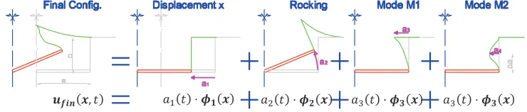
In order to reach this objective, in this paper we propose a simplified model of a soil-structure interface where only the lateral interface with the soil is considered flexible (the basemat remains rigid and no constraint for the lateral wall). We propose 4 modes (Figure 4) to represent the kinematic field of the interface:
.
Figure 4: Decomposition for the motion for a flexible foundation.
The analytical expression for each mode ࣘ is expressed as follows:
൜ࣘ ࣘሺݔǡ ݕǡ ݖሻ ൌ ͳ ڄ ࢋෞ࢞
ሺݔǡ ݕǡ ݖሻ ൌ െሺݖെ ݖ௦ሻ ڄ ࢋෞ ሺݔ࢞ െ ݔ௦ሻ ڄ ࢋෞቊࢠ
ࣘሺݔǡ ݕǡ ݖሻ ൌ ͳ െ ሺߨ൫ݖെ ݖ൯Ȁʹܦሻڄ ࢋෞ࢞
ࣘሺݔǡ ݕǡ ݖሻ ൌ ͳ െ ሺߨ൫ݖെ ݖ൯Ȁܦሻ ڄ ࢋෞࢠ
where ݔ௦ and ݖ௦ are the coordinates of the basemat center.
Thus the transfer functions (TFs), with respect to the input motion ܣ at the free field surface level, can be expressed as follows:
ቐܷ
ሺ߱ሻ ൌ ݂݂ݐ൫ܽሷ
ଵሺݐሻ൯Ȁ݂݂ݐ ቀܣሺݐሻቁ
ȣሺ߱ሻ ൌ ݂݂ݐ൫ܽሷଶሺݐሻ൯Ȁ݂݂ݐ ቀܣሺݐሻቁ
ቐͳ
ሺ߱ሻ ൌ ݂݂ݐ൫ܽሷ
ଷሺݐሻ൯Ȁ݂݂ݐ ቀܣሺݐሻቁ
ʹሺ߱ሻ ൌ ݂݂ݐ൫ܽሷସሺݐሻ൯Ȁ݂݂ݐ ቀܣሺݐሻቁ
(18)
Using a FEM model, the transfer functions of several foundation geometries have been calculated and plotted in Figure 5. It is easy to see that, in their dimensionless form, the transfer functions (17) of an interface (radius ܴ, embedmentܦ), representing the kinematic interaction, have the same forms (only the rocking TF, Figure 5(b), shows a dependence on the ratio ܦȀܴ for high frequencies).
Similarly to the Kausel approach, we define an approximate transfer function for each mode. The construction of these functions is carried out using a classical method based on error reduction:
ܷሺ߱ሻ ൌ ൞
ቀଶఠగఠ
ቁ ݂݅߱ ͲǤ߱
ቊͳ ቂͳǤͳͺ͵ͻ െ ͲǤͲʹʹͺఠఠ
ቃ ڄ ቤ ቆߨ ቀͳ
ఠିǤఠ
ଵǤଽସସఠቁቇቤ ͲǤͲͶʹʹ ቀ
ఠ
ఠെ ͳቁቋ ͲǤͶͷ͵݂݅߱ ͲǤ߱
(19)
ȣሺ߱ሻ ൌ ൞ͲǤʹͷ ቂͳ െ ቀ గఠ
ఠቁቃ Ȁܴ݂݅߱ ͲǤͷ߱
ͲǤʹͷ ቊͳ ቂͳǤ͵ʹͻʹ െ ͲǤͲʹͷఠఠቃ ڄ ቤ ቆగଶቀͳ ఠିǤହఠ
Ǥ଼ଶଶఠቁቇቤ െ ͲǤͲ͵ͳͳ ቀ
ఠ
ఠെ ͲǤͷቁቋ Ȁܴ݂݅߱ ͲǤͷ߱
(20)
ͳሺ߱ሻ ൌ ൞
ʹǤ͵͵ ቂͳ െ ቀଶఠగఠቁቃ ݂݅߱ ߱
ቀʹǤͷͻ െఠఠ
ቁ ڄ ቤ ቆ
గ ଶቀͳ
ఠିఠ
ସǤସଽସସఠቁቇቤ ͲǤͲͶͳ ቀ
ఠ
ఠെ ͳቁ ݂݅߱ ߱
(21)
ʹሺ߱ሻ ൌ
ە ۖ ۔ ۖ
ۓͲǤͷ כ ቚ ቀߨଵǤଽଵଵఠఠ ቁቚ ͲǤͳͲʹͺ
ఠ
ఠݏ݅߱ ͳǤͻͳͳ߱
ͳǤͺͶͶͶ ቤ ቆߨ ቀఠିଵǤଽଵଵఠ
ଷǤ଼ଽఠ ቁቇቤ ͲǤͳͲʹͺ
ఠ
ఠ݂݅ͳǤͻͳͳ߱൏ ߱ ͷ߱
ͲǤͷͳͶ݂݅߱ ͷ߱
(22)
where ߱ൌ ʹߨܸ௦ȀሺͶܦሻ and ܸ௦ is the soil shear wave velocity.
For a real soil-structure interface, the transfer functions are defined as a linear interpolation between these of the rigid foundation proposed by Kausel (Equations 15, 16) and those of the foundation with a totally flexible lateral wall (Equations (19) ~ (22)):
ܷ ሺ߱ሻ ൌ ߙܷሺ߱ሻ ሺͳ െ ߙሻܷሺ߱ሻ (23)
ȣ ሺ߱ሻ ൌ ߙȣሺ߱ሻ ሺͳ െ ߙሻȣሺ߱ሻ (24)
ͳሺ߱ሻ ൌ ሺͳ െ ߙሻͳሺ߱ሻ (25)
ʹሺ߱ሻ ൌ ሺͳ െ ߙሻʹሺ߱ሻ (26)
where ߙ ൌாೢೢோ
ாೞڄுȀ ቀͳ
ாೢೢோ
ாೞڄுቁ is a dimensionless parameter. In this expression, ܧ௪ is the Young’s
Figure 5. Approximated transfer functions of the horizontal displacement (a), rocking (b), Mode M1 (c) and Mode M2 (d) for a totally flexible interface with respect to the normalised frequency (߱Ȁ߱).
NUMERICAL CASE
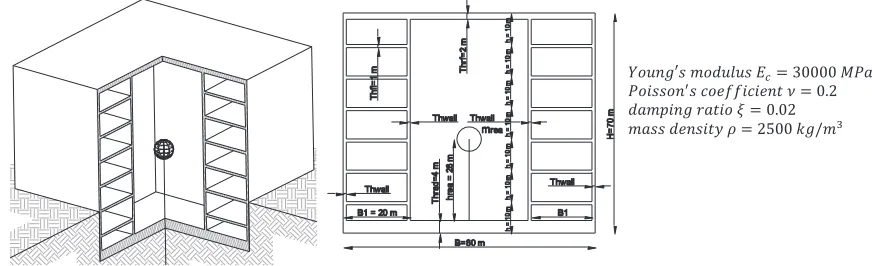
In order to validate the proposed model, we have conducted a numerical study on the response of a simplified model of a reactor building under seismic loading where the SSI has been taken into account. The structure model, shown in Figure 6, is a regular structure both horizontally and vertically. The main dimensions are ܮ ൌ ͺͲ݉ (length) x ܤ ൌ ͺͲ݉ (width) x ܪ ൌ Ͳ݉ (height). The reactor building (RB) is embedded in the soil by means of its foundation with an embedment depth ܦ equal to ʹͲ݉. The mechanical properties are also shown in Figure 7.
Figure 6. Structure model.
The basemat and roof slab thicknesses are 4 m and 2 m respectively. The thickness of all walls (internal and external) is equal to ͳǤͷ݉. To represent the internal structures (i.e. nuclear reactor, steam generators etc.), a vertical beam-lumped mass system is considered at the center of the structure (mass݉ ൌ ͵ͲͲͲͲݐand height݄ ൌ ʹ݉). The vertical beam is massless and clamped on the foundation. The mass is connected to a flexible beam, constrained to move only in the horizontal directions. The bending stiffness of the beam is tuned so that the frequency of the above oscillator is equal to 8 Hz which is a reasonable value for the first frequency of the internal structures. A second containment wall separates the structure into two parts: the interior/central part and the external part. The peripheral part of the structure is divided into seven stories with six regularly spaced 1 m thick floors as shown in Figure 6.
ܻݑ݊݃Ԣݏ݉݀ݑ݈ݑݏܧൌ ͵ͲͲͲͲܯܲܽ
ܲ݅ݏݏ݊ᇱݏ݂݂ܿ݁݅ܿ݅݁݊ݐߥ ൌ ͲǤʹ
݀ܽ݉݅݊݃ݎܽݐ݅ߦ ൌ ͲǤͲʹ
The structure is embedded in a multi-layered soil characterized by its shear wave velocity ܸ௦ǡଷ ൌ ͵ͲȀ൫σ ൫݄ேୀଵ Ȁܸ௦ǡ൯൯, where N is the number of layers within the first 30 m of depth. The mechanical
properties are shown in Figure 7.
Figure 7. Geotechnical profile of the soil.
In this study, the structure and the soil are considered to be elastic. As for the seismic input motion, a synthetic signal is introduced at the level of the free field surface (Figure 8).
Figure 8. Seismic loading.
The first step of this numerical study is to define the impedance functions of the soil-structure interface considered as rigid and massless. In the theoretical part, we didn’t specify if the proposed calibration method could be used for multi-layered soil or only for homogenous soil. In principle, there is no limitation but in the case of the multi-layered soil, the impedances functions are less smooth then in the homogenous case. Thus, using only three parameters, it could be difficult to ensure a calibration in an optimally way.
Figure 9. Comparison of the impedance functions between a FEM model and the simplified approach -horizontal impedance, real part (a) and imaginary part (b)
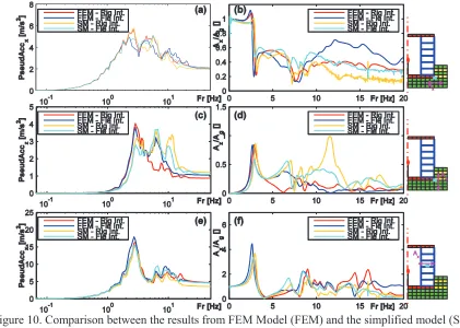
We compare in Figure 10 the results obtained from a “full FEM” model and from our approach concerning two kinematic conditions for the soil-structure interface: rigid interface and rigid basemat with flexible lateral foundation wall. The evaluation of the FIM has been carried out using the Kausel approach for the rigid case and our approach for the flexible one. In the preceding section, the formulation for the transfer function has been done regarding a foundation founded in a homogenous half-space. But now, we analyse a reactor building sitting on a multilayered soil. Several tests have shown that for a regular variation of the mechanical proprieties of soil with respect to depth, the Kausel method and our approach are able to represent the movement of the interface. However, the discrepancies are more important for the high dimensionless frequencies.
Figure 10. Comparison between the results from FEM Model (FEM) and the simplified model (SM). Horizontal response spectre (a) and horizontal TF (b) at the basemat level –
We observe in Figure 10 a good accordance between the results of the two models. More specifically, we can note that:
· in the case of a rigid foundation (red and orange lines, Figure 10), the simplified model is able to represent the dynamic stiffness of the interface. We can notice a slight frequency shift (Figure 10(e) and 10(f)) and an underestimation of the 4th floor response which can be attributed to the calibration of the damping terms. Regarding the vertical response of the basemat, an amplification for the high frequencies is observed that can be generated by the choice of calibration frequencies. Concerning the Foundation Input Motion (FIM), the Kausel approach seems to compute very well the motion of the basemat (Figure 10(a) and 10(b)) except for the high frequencies where the FIM is under-estimated;
· in the case of a flexible foundation (bleu and cyan lines, Figure 10), the frequency shift is more apparent (Figure 10(e) and 10(f)) and the underestimation is still present. Regarding the FIM, our model seems to give a good approximation, but in the high frequency range the accordance is not as good.
CONCLUSION
In conclusion, we have defined a new simplified model for the flexible soil-structure interfaces based on the Wolf (1988) approach. In addition, a method for the estimation of the Foundation Input Motion (FIM) has been proposed. These approaches seem to give good numerical results. However, several aspects need to be further analysed:
· The repartition for the stiffness, mass and damping, to each point of the interface, has been performed using Equations (4), (5) and (6). In this simple form, there is no conditions which can guarantee the stability of the model on every interface point (positive damping value, for example);
· The deduction of the FIM motion doesn’t take into account the influence of the soil damping. This can influence the kinematic interaction, especially for the high dimensionless frequencies;
· The proposed model, used to represent the dynamic stiffness of the interface, is very simple. Thus the number of points used to approximate the impedance functions is limited and doesn’t allow a good calibration in the case of a large frequency interval.
REFERENCES
Chabas F. and Soize C. (1987). “Modelling mechanical subsystem by boundary impedance in finite element method”, La Recherche Aerospatiale (English version), 5 59-75.
Cotterau R., Clouteau D., Soize C. (2007). « Construction of a probabilistic model for impedance matrices », Computer Methods in Applied Mechanics and Engineering, 196 2252-2268.
Grange S., Kotronis P.and Mazars J. (2009). “A macro-element to simulate 3D soil–structure interaction considering plasticity and uplift”, International Journal of Solids and Structures,46 3651-3663 Kausel E., Whitman R. V. and Morray J. P. (1978). “The spring method for embedded Foundation,”
Nuclear Engeneering and Desing, 48 377-392
Kurimoto O. and Iguchi M. (1996). “Evaluation of foundation input motion based on observed seismic motions,” Paper No 317 Eleventh World Conference on Earthquake Engineering, Elsevier Science, Acapulco, Mexico.
Cremer C., Pecker A. and Davenne L. (2001). “Cyclic macro-element for soil–structure interaction: material and geometrical non-linearities”, “International Journal for Numerical and Analytical
Methods in Geomechanics,” 25 1257-1284.