ABSTRACT
ZHENG, JUNYU. Quantification of Variability and Uncertainty in Emission Estimation: General Methodology and Software Implementation.(Under the supervision of Dr. H. Christopher Frey).
methodologies and algorithms presented in this dissertation for variability and uncertainty analysis. The tool can be used in any quantitative analysis fields where variability and uncertainty analysis are needed in model inputs.
To my beloved parents, Yongnian Zheng and Guifang Zhang for their constant understanding and support
BIOGRAPHY
Junyu Zheng received his Bachelor of Engineering degree in Water Supply and Drainage from Wuhan Urban Construction Institute, Wuhan, China, in 1991. During the period of August of 1991 through August of 1993, he worked as a water supply process manager in Power Plant, Beijing Yanshan Petrol & Chemical Corporation (BYPCC), where he was responsible for process management of industrial and civil water supply of BYPCC.
Junyu Zheng was admitted to the Department of Environmental Engineering of Tsinghua University, China, in September of 1993 for his pursuit of master degree, where he worked as research assistant at the Environmental System Lab and his research focused on the probabilistic analysis of water quality model. He earned his Master of Science degree in Environmental Engineering from Tsinghua University in 1996. After he received his M.S degree, he accepted a position of real-estate appraiser from Jingdu Certified Public Accountant (one member of Horwath International), Beijing, and part-time worked as an assistant general manager and software developer at Beijing Kelier Information Inc. to engage in the software development and network installation of Automatic Check Telephone Query System.
Junyu Zheng came to North Carolina State University, Raleigh, North Carolina, USA, in August 1998 for his Ph.D. in Environmental Engineering program. During his Ph.D study, he worked as a research assistant at the Computational Laboratory for Energy, Air and Risk (CLEAR).
ACKNOWLEDGEMENTS
This research was supported by U.S. EPA STAR Grants Nos. R826766 and R826790. The ORD of U.S. EPA funded the development of AuvTool via contract ID-S794-NTEX.
The author wishes to express his appreciation to Dr. H. Christopher Frey for his constant inspiration and guidance throughout the course of this research. Appreciation is also extended to Drs. L.A. Stefanski, E.D. Brill, J. W. Baugh, D. Vandervaart and A. Anton for their valuable suggestions. The author appreciates the guidance and encouragement of Dr. Jianping Xue and Dr. Haluk Ozkaynak of U.S. EPA during the development of the AuvTool.
Table of Contents
LIST OF TABLES... xii
LIST OF FIGURES ... xiv
PART I INTRODUCTION... 1
1.0 Introduction... 3
1.1 Variability ... 5
1.2 Uncertainty... 6
1.3 Distinctions Between Variability and Uncertainty ... 8
1.4 Examples of Probabilistic Analysis ... 10
1.5 Limitations of Current Studies in Variability and Uncertainty Analysis.. 11
1.6 Available Software Tools in Probabilistic Analysis ... 14
1.7 Objectives ... 15
1.8 Overview of Research... 16
1.9 Organization... 18
1.10 References... 20
PART II GENERAL METHODLOGY OF QUANTIFICATION OF VARIABILITY AND UNCERTAINTY IN EMISSION ESTIMATION ... 25
2.0 General Methodology ... 27
2.1 General Approach for Developing a Probabilistic Emission Inventory ... 28
2.2 Data Preparation... 29
2.3 Emission Inventory Models ... 30
2.4 Numerical sampling techniques... 32
2.4.1 Monte Carlo Sampling... 32
2.4.3 Latin Hypercube Sampling ... 34
2.5 Visualization of Datasets Using Empirical Distributions ... 35
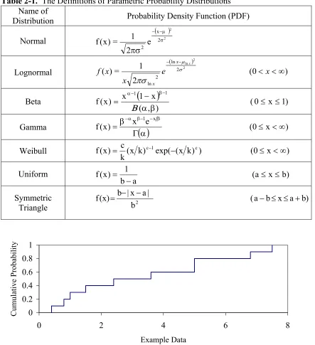
2.6 Definitions of Probability Distribution Models ... 38
2.6.2 Empirical Distribution ... 39
2.7 Parameter Estimation of Parameter Distributions... 40
2.7.1 Method of Matching Moments ... 43
2.7.2 Maximum Likelihood Estimation (MLE)... 43
2.8 Evaluation of Goodness-of-Fit of a Probability Distribution Model ... 47
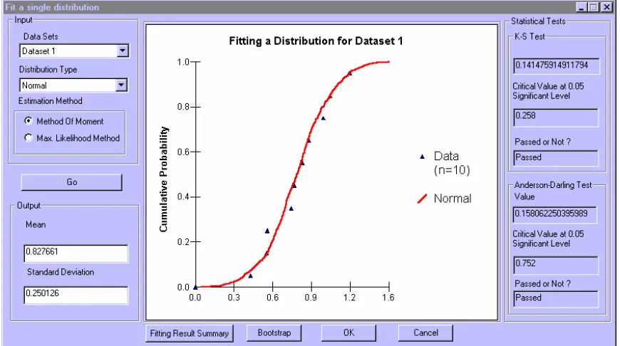
2.8.1 Graphical Comparison of CDF of Fitted Distribution to the Data ... 50
2.8.2 Kolmogorov-Smirnov Test ... 51
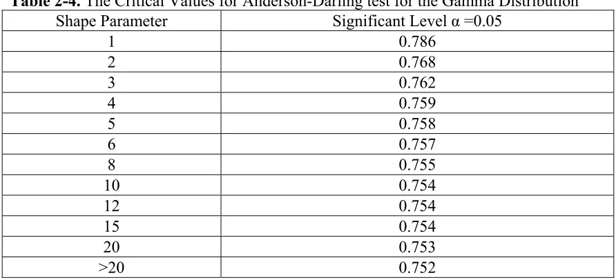
2.8.3 Anderson-Darling Test... 54
2.8.4 Graphical Comparison of Confidence Intervals for CDF of Fitted Distribution to the Data ... 56
2.8.5 Summary of Methods for Evaluating Goodness-of-Fit ... 57
2.9 Algorithms for Generating Random Samples from Probability Distributions... 58
2.9.1 Pseudo Random Number Generator ... 59
2.9.2 Empirical Distribution ... 60
2.10 Characterization of Uncertainty in the Distribution for Variability... 61
2.10.1 Bootstrap Method... 63
2.10.2 Methods of Generating Bootstrap Samples ... 64
2.10.3 Methods of Forming Bootstrap Confidence Intervals ... 65
2.10.4 Two-Dimensional Simulation of Variability and Uncertainty... 69
2.11 Probabilistic Approaches for Simulating Variability and Uncertainty in the Emission Inventories... 72
2.12 Identification of Key Sources of Variability and Uncertainty ... 73
2.13 Summary ... 76
2.14 References... 78
PART III SOFTWARE IMPLEMENTATION ... 81
3.0 Software Implementation... 83
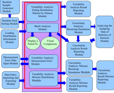
3.1 Software Implementation of AuvTool ... 83
3.1.1 AuvTool Software Design Considerations ... 84
3.1.2 Development Environment and Tools ... 84
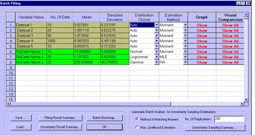
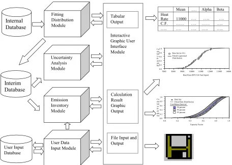
3.1.4 AuvTool Main Modules... 85
3.2 Software Implementation of AUVEE... 98
3.2.1 General Structure of the AUVEE Prototype Software ... 98
3.2.2 Databases in the AUVEE Prototype Software... 98
3.2.3 Modules in the AUVEE Prototype Software ... 100
3.2.4 Software Development Tools ... 102
3.3 References... 104
PART IV QUANTIFICATION OF VARIABILITY AND UNCERTAINTY USING MIXTURE DISTRIBUTION: EVALUATION OF SAMPLE SIZE, MIXING WEIGHTS AND SEPARATION BETWEEN COMPONENTS ... 105
Abstract... 107
1.0 Introduction... 108
2.0 Methodology... 113
2.1 Mixture Distribution ... 113
2.2 Parameter Estimation of Mixture Distributions... 115
2.3 Quantification of Variability and Uncertainty Using Mixture Distribution ... 118
3.0 Introduction to Study Design... 122
4.0 Results and Discussion ... 123
4.1 Properties of Confidence Intervals of Cumulative Distributions.... 123
4.2 Comparisons between Single Distribution and Mixture Distributions... 125
4.3 Dependencies among Sampling Distributions of Parameters of Mixture Distributions... 127
5.0 An Illustrative Case Study: NOx Emission Factor for a Coal-Fired of Power Plant ... 128
5.1 Parameter Estimation for the Fitted Distribution... 129
5.2 Variability and Uncertainty in the NOx Emission Factor ... 129
5.3 Uncertainty in the Mean NOx Emission Factor ... 130
6.0 Conclusion ... 131
PART V QUANTIFICATION OF VARIABILITY AND UNCERTAINTY
WITH MEASUREMENT ERROR ... 151
Abstract... 153
1.0 Introductuion... 154
1.1 Variability and Uncertainty... 155
1.2 Limitations of Current Studies in Variability and Uncertainty Analysis... 155
1.3 Measurement Error and Uncertainty... 156
1.4 Classification of Measurement Errors ... 157
1.5 Purpose of This Study... 158
2.0 Methodology... 158
2.1 Measurement Error Models ... 159
2.2 Error Free Data Construction... 160
2.3 Quantification of Variability and Uncertainty with Measurement Error ... 162
3.0 Introduction to Study Design... 167
3.0 Case Study ... 167
4.0 Conclusion ... 172
Acknowledgements... 174
References... 175
PART VI QUANTIFICATION OF VARIABILITY AND UNCERTAINTY IN AIR POLLUTANT EMISSION INVENTORIES: METHOD AND CASE STUDY FOR UTILITY NOX EMISSIONS... 187
Abstract... 189
Implications... 190
1.0 Introduction... 190
2.0 Methodology... 193
2.1 Compilation and Evaluation of a Database... 193
2.2 Visualization of Data ... 196
2.3 Fitting, Evaluating, and Selecting Parametric Probabilistic Distribution Models ... 197
2.5 Propagation of Uncertainty and Variability through a Model ... 200
2.6 Identifying Key Sources of Uncertainty ... 201
3.0 Introduction to AUVEE ... 202
4.0 Case Study: A Probabilistic Emission Inventory for Utilities in a Single State... 204
5.0 Conclusions... 210
Acknowledgments... 213
References... 214
About the Authors... 226
PART VII PROBABILISTIC ANALYSIS OF DRIVING CYCLE-BASED HIGHWAY VEHICLE EMISSION FACTORS ... 227
Abstract... 229
1.0 Introduction... 230
1.1 Sources of Variability and Uncertainty... 231
1.2 Variability and Uncertainty in Highway Vehicle Emission Factors... 232
1.3 Modeling Assumptions and Input Data ... 232
1.4 Brief Review of the Mobile5b Model... 232
1.5 Simplified Probabilistic Emission Factor Model... 233
1.6 Collection of Emission Test Data ... 235
2.0 Quantification of Inter-Vehicle Variability in Correction Factors ... 236
3.0 Quantification of Uncertainty in Mean Correction Factors ... 240
4.0 Quantification of Variability and Uncertainty in the Emission Factors . 242 4.1 Inter-Vehicle Variability in Emission Factors. ... 243
4.2 Uncertainty in Mean Emission Factors... 245
4.3 Identifying Key Sources of Uncertainty ... 246
5.0 Results and Discussion ... 247
6.0 Acknowledgments... 249
7.0 References... 250
PART VIII CONCLUSIONS AND RECOMMENDATIONS ... 275
8.1.1 Methodologies... 278
8.1.2 Case Studies ... 280
8.1.3 Software Development... 281
8.2 Conclusions... 282
8.2.1 Methodological Conclusions ... 282
8.2.2 Conclusions Based Upon Case Studies... 284
8.3 Recommendations for Future Work... 286
8.3.1 Methodologies... 286
8.3.2 Probabilistic Emission Inventories ... 287
8.3.3 Development of AuvTool ... 288
APPENDIX A... 293
List of Tables
PART II
Table 2-1. The Definitions of Parametric Probability Distributions... 40 Table 2-2. Citical Value of Dnα the Kolmogorov-Smirnov Test... 53 Table 2-3. The Critical Values for Anderson-Darling test for Normal, Lognormal
and Weibull distributions... 55 Table 2-4. The Critical Values for Anderson-Darling test for the Gamma Distribution.. 55 PART III
Table 3-1. AuvTool Function Module Summarization Table ... 87 PART IV
Table 1. Selected Population Mixture Lognormal Distributions with Two
Components ... 136 Table 2. Comparison of 95% Confidence Intervals of Selected Statistics of Single
and Two Component Mixture Lognormal Distributions Fitted to Mixture Populations with Varying Component Separation and Standard Deviation for n=100 and w=0.3... 137 Table 3. Comparison of 95% Confidence Intervals of Selected Statistics of Single
and Two Component Mixture Lognormal Distributions Fitted to Mixture Populations with Varying Component Separation and Standard Deviation for n=100 and w=0.5... 138 Table 4. Uncertainty of Estimated Parameters of the Fitted Mixture Lognormal
Distribution ... 136 PART V
Table 1. The Observed Data Set and Estimated Error Free Data Sets under Different Measurement Error Models ... 178 Table 2. The Fitted Lognormal Distributions under Different Measurement Error
Models ... 179 Table 3. Uncertainty in the Mean under Different Measurement Error Models ... 179 PART VI
Table 1. Summary of 12-Month NOx Emission and Activity Factors and of Fitted
Table 2. Summary of Uncertainty Results for the Emission Inventory Case Study... 219
PART VII Table 1. Characterization of Inter-Vehicle Variability in Estimated Tailpipe CO Emission Factors for Technology Group 8... 252
Table 2. Characterization of Fleet Average Uncertainty in Estimated Tailpipe CO Emission Factors for Technology Group 8... 253
Table S-2. Input Uncertainty Assumptions for CO Emissions... 257
Table S-3. Input Variability Assumptions for HC Emissions... 258
Table S-4. Input Uncertainty Assumptions for HC Emissions... 259
Table S-5. Input Variability Assumptions for NOx Emissions ... 260
Table S-6. Input Uncertainty Assumptions for NOx Emissions ... 261
Table S-7. Characterization of Inter-Vehicle Variability in Estimated Tailpipe HC Emission Factors for Technology Group 8... 262
Table S-8. Characterization of Fleet Average Uncertainty in Estimated Tailpipe HC Emission Factors for Technology Group 8... 263
Table S-9. Characterization of Inter-Vehicle Variability in Estimated Tailpipe NOx Emission Factors for Technology Group 8... 264
Table S-10. Characterization of Fleet Average Uncertainty in Estimated Tailpipe NOx Emission Factors for Technology Group 8... 265
Table S-11. Correlation of Uncertain CO Emission Factor with Input Uncertainties .... 266
List of Figures
PART II
Figure 2-1. Plot Illustrating the 95 Percent Probability Range on a Cumulative
Distribution Function. ... 36 Figure 2-2. Example Graph of Visualizing Data Using the Hazen’s Plotting Position
Method (n=10)... 37 Figure 2-3. An example of an Empirical Distribution Represented a Step Function
(n=10) ... 40 Figure 2-4. Comparison of Fitted Beta Distribution to an Example Dataset... 51 Figure 2-5. An Illustrative Example of Graphical Comparison of Confidence Intervals
for CDF of Fitted Distribution to the Data ... 56 Figure 2-6. Flow Diagram For Bootstrap Simulation and Two-Dimensional Simulation
of Variability and Uncertainty. (Where: B=number of Bootstrap
Replications, q=Sample Size Used for Uncertainty, p=Sample Size Used of Variability)... 71 PART III
Figure 3-1. The Conceptual Structure Design and Context Diagram of AuvTool
System ... 86 Figure 3-3a. Batch Analysis Module (1)... 91 Figure 3-3b. Batch Analysis Module (2) ... 91 Figure 3-4. Conceptual Structure Design of the Analysis of Uncertainty and
Variability in Emissions Estimation (AUVEE) Prototype Software... 99 PART IV
Figure 1. Simplified Flow Diagram for Quantification of Variability and Uncertainty Using Bootstrap Simulation based upon Mixture Distributions ... 139 Figure 2. 95 Percent Confidence Intervals of Cumulative Distribution of Two
Component Lognormal Distributions Fitted to a Mixture Population Distribution (µ1=1.0, σ1=0.5, µ2=1.5, σ2=0.5) for n=25,50 and 100, for
w=0.1,0.3 and 0.5 Based on Bootstrap Simulation (B=500)... 140 Figure 3. 95 Percent Confidence Intervals of Cumulative Distribution of Two
Component Lognormal Distributions Fitted to a Mixture Population Distribution (µ1=1.0, σ1=0.5, µ2=2.0, σ2=0.5) for n=25,50 and 100, for
w=0.1,0.3 and 0.5 Based on Bootstrap Simulation (B=500)... 141 Figure 4. 95 Percent Confidence Intervals of Cumulative Distribution of Two
Distribution (µ1=1.0, σ1=0.5, µ2=3.0, σ2=0.5) for n=25,50 and 100, for
w=0.1,0.3 and 0.5 Based on Bootstrap Simulation (B=500)... 142 Figure 5. 95 Percent Confidence Intervals of Cumulative Distribution of Two
Component Lognormal Distributions Fitted to a Mixture Population Distribution (µ1=1.0, σ1=0.5, µ2=6.0, σ2=0.5) for n=25,50 and 100, for
w=0.1,0.3 and 0.5 Based on Bootstrap Simulation (B=500)... 143 Figure 6. 95 Percent Confidence Intervals of Cumulative Distributions of a Single
Lognormal Distribution Fitted to a Mixture Population Distribution (µ1=1.0,
σ1=0.5, µ2=1.5, σ2=0.5) for n=25,50 and 100, for w=0.1,0.3 and 0.5 Based on Bootstrap Simulation (B=500)... 144 Figure 7. 95 Percent Confidence Intervals of Cumulative Distributions of a Single
Lognormal Distribution Fitted to a Mixture Population Distribution (µ1=1.0,
σ1=0.5, µ2=2.0, σ2=0.5) for n=25,50 and 100, for w=0.1,0.3 and 0.5 Based on Bootstrap Simulation (B=500)... 145 Figure 9. Scatter Plots of Bootstrap Simulation (B=500) Results for Parameters of Two
Component Lognormal Mixture Distributions for n=100, w=0.5 with
Moderately Separated Components (µ1=1.0, σ1=0.5, µ2=3.0, σ2=0.5). ... 147 Figure 10. Scatter Plots of Bootstrap Simulation (B=500) Results for Parameters of
Two Component Lognormal Mixture Distributions for n=100, w=0.5 with highly Separated Components (µ1=1.0, σ1=0.5, µ2=6.0, σ2=0.5). ... 148 Figure 11. Mixture lognormal distribution fitted to six-month average NOx emission
factor data for T/LNC1 technology group (n=41)... 149 Figure 12. Probability band for fitted mixture lognormal distribution. ... 149 PART V
Figure 1. Flow Diagram for Characterizing Variability and Uncertainty with
Measurement Error by Using the Bootstrap Pair Technique ... 165 Figure 2. The Fitted Lognormal Distributions to the Error Free Data Set under
Different Measurement Errors and the Observed Data Set... 180 Figure 3. The Probability Band Based upon the Fitted Lognormal Distribution to the
Observed Data Set (no measurement error is assumed)... 180 Figure 4. The Probability Band Based upon the Fitted Lognormal Distribution to the
Error Free Data at σe=10.0 without the Inclusion of Measurement Error... 181 Figure 5. The Probability Band Based upon the Fitted Lognormal Distribution to the
Error Free Data at σe=10.0 with the Inclusion of Measurement Error ... 181 Figure 6. The Probability Band Based upon the Fitted Lognormal Distribution to the
Error Free Data at σe=20.0 without the Inclusion of Measurement Error... 182 Figure 7. The Probability Band Based upon the Fitted Lognormal Distribution to the
Figure 8. The Probability Band Based upon the Fitted Lognormal Distribution to the Error Free Data at σe=40.0 without the Inclusion of Measurement Error... 183 Figure 9. The Probability Band Based upon the Fitted Lognormal Distribution to the
Error Free Data at σe=40.0 with the Inclusion of Measurement Error ... 183 Figure 10. The Probability Band Based upon the Fitted Lognormal Distribution to the
Error Free Data at σe=55.5 without the Inclusion of Measurement Error... 184 Figure 11. The Probability Band Based upon the Fitted Lognormal Distribution to the
Error Free Data at σe=55.5 with the Inclusion of Measurement Error ... 184 Figure 12. The Sampling Distributions for the Mean under Different Measurement
Error Models... 185 PART VI
Figure 1. Scatter plot of 12-month NOx Emission Rate of 1997 and 1998 (No. of
Data=390)... 220 Figure 2. Scatter Plot for 12-month Average Heat Rate versus 12-month Average
Capacity Factor for Tangential-Fired Boilers Using Low NOx Burners and OverfireAir Option 1. (n=36) ... 220 Figure 3. Conceptual Design of the Analysis of Uncertainty and Variability in
Emissions Estimation (AUVEE) Prototype Software. ... 221 Figure 4. Probability Band for Distribution Fitted to Example Heat Rate Data for
Dry Bottom Wall-fired Boilers Using Low NOx Burners (n=98) ... 222 Figure 5. Probability Band for Distribution Fitted to Example Capacity Factor Data
for Dry Bottom Wall-fired Boilers Using Low NOx Burners (n=98) ... 222 Figure 6. Probability Band for Distribution Fitted to Example NOx Emission Rate
Data for Dry Bottom Wall-fired Boilers Using Low NOx Burners (n=98).... 223 Figure 7. Probability Bands Based Upon Number of Units in the Emission Inventory
(n=3) for the Example of NOx Emission Rate... 223 Figure 8. Uncertainty in a 12-Month NOx Emission Inventory for an Individual
Technology Group Comprised of 3 Units. ... 224 Figure 9. Uncertainty in a 12-Month NOx Emission Inventory Inclusive of Four
Technology Groups. ... 224 Figure 10. Relative Importance of Uncertainty in Emissions from Individual
Technology Groups with Respect to Overall Uncertainty in the Total
PART VII
Figure 1. Estimated Inter-Vehicle Variability in Temperature Correction Factor For CO Technology Group 8 ... 254 Figure 2. Estimated Fleet Average in Temperature Correction Factor For CO
Technology Group 8... 254 Figure S-1. Estimated Inter-Vehicle Variability in Temperature Correction Factor For
HC Technology Group 8 ... 269 Figure S-2. Estimated Fleet Average in Temperature Correction Factor For HC
Technology Group 8... 269 Figure S-3. Estimated Inter-Vehicle Variability in Temperature Correction Factor
For NOx Technology Group 8 ... 270 Figure S-4. Estimated Fleet Average in Temperature Correction Factor For NOx
Technology Group 8... 270 Figure S-5. Estimated Inter-Vehicle Variability in RVP Correction Factor For CO
Technology Group 8... 271 Figure S-6. Estimated Fleet Average in RVP Correction Factor For CO Technology
Group 8... 271 Figure S-7. Estimated Inter-Vehicle Variability in RVP Correction Factor For NOx
Technology Group 8... 272 Figure S-8. Estimated Fleet Average in RVP Correction Factor For NOx Technology
Group 8... 272 Figure S-9. Estimated Inter-Vehicle Variability in RVP Correction Factor For HC
Technology Group 8... 273 Figure S-10. Estimated Fleet Average in RVP Correction Factor For HC
Technology Group 8... 273 APPENDIX A
PART I
INTRODUCTION
1.0 Introduction
Air pollutant emission inventories (EIs) are a vital component of environmental decision-making. They are often used for short-term or long-term emission trend characterization, emission budgeting for regulatory and compliance purposes, and the predication of ambient pollutant concentrations using air quality models. If random errors and biases in emission inventories are not quantified, they can lead to erroneous conclusions regarding trends in emissions, source apportionment, compliance, and the relationship between emissions and ambient air quality (Frey et al., 1999). For example, if resources are mistakenly devoted to reduce emissions for a source category where emissions are overestimated, or if resources are not applied to reduce emissions from a source category where emissions are under-estimated, then air quality objectives cannot be achieved in an efficient and cost-effective manner.
In practice, an emission inventory is often obtained from emission factors multiplied by activity factors. Emission factors are typically assumed to be
representative of an average emission rate from a population of pollutant sources in a specific category (EPA,1995). For example, a power plant emission factor can be an average emission rate among all of the power plant units of the same type within a state. However, there may be uncertainty in the population average emission rates because of random sampling error, measurement errors, or possibly because the sample of power plants from which the emission factor was developed was not a representative sample. These errors in the estimation of the emission factor or activity factor can lead to biases in emission inventory estimation.
Some qualitative analysis methods have been presented in the past years,
(DARS) to address the errors in the estimation of the emission factor or activity factor. For example, in the data quality rating methods, qualitative “A” through “E” ratings are defined and reported in EPA’s Compilation of Air Pollutant Emission Factors (EPA, 1995). DARS is a method for combining data quality scores for both emission factor and activity data to develop an overall quality score for an emission inventory (Beck and Wilson, 1997). While DARS can be used to compare quality ratings for EIs, it can neither be used to quantify the precision of an inventory nor to evaluate the robustness of a decision to uncertainty. Other efforts have been focused on characterizing the mean and variance of emission estimates and using simplified approaches for combining
uncertainties in activity and emission factor data to arrive at an aggregate uncertainty estimate (Dickinson and Hobbs, 1989; NRC 1991; Balentine and Dickinson, 1995). The applications of these approaches suffer from many shortcomings including: restrictive assumptions about the shape of probability distribution models; failure to deal with dependences between uncertainty estimates; failure to distinguish between variability and uncertainty estimates; inappropriate averaging times; improperly analyzed small sample data; and failure to use proper protocols in eliciting expert judgments.
The use of quantitative methods for dealing with variability and uncertainty is becoming more widely recognized and recommended for environmental modeling and assessment applications. For example, the National Research Council recently released a report on mobile source emissions estimation that calls for new efforts to quantify
Carlo simulation methods (EPA, 1997, 1999a), has developed a guideline document on Monte Carlo methods (EPA, 1996) and has included guidance regarding probabilistic analysis in its most recent draft of Risk Assessment Guidance for Superfund (EPA, 1999b). One of the recommendations of the Emission Inventory Improvement Program (EIIP) of the US EPA is to encourage the use of quantitative methods to characterize variability and uncertainties in emission inventories (Radian, 1996). Uncertainty analysis is now part of the planning process for major assessments performed by EPA, such as the National Air Toxics Assessment.
The Intergovernmental Panel on Climate Change (IPCC) recently issues a good practice document regarding uncertainty analysis for greenhouse gas emission inventories (IPCC, 2000).
1.1 Variability
Variability is the heterogeneity of a quantity over time, space or members of a population. Thus variability indicates the range that a quantity can vary over.
by a frequency distribution showing the variation in a characteristic of interest over time, space. Knowledge of the frequency distribution helps to assess whether a population needs to be subdivided into groups which are more nearly homogeneous. (Frey,1997; Cullen, Frey, 1999; Morgan and Henrion,1990)
1.2 Uncertainty
Uncertainty refers to a lack of knowledge about the true value of a quantity. Uncertainty can be quantified as a probability distribution representing the likelihood that the unknown quantity falls within a given range of values (Cullen and Frey, 1999). Uncertainty can be introduced in every step of analyzing a quantity. For example, it can come from measurement error because of biases in the measuring apparatus and the experimental procedures or from human error, such as random mistakes in recording or processing data; and random sampling error. Uncertainty exists in the whole model building process (Cullen and Frey, 1999). Draper et al. (1987) and Hodges (1987) pointed out that there are typically three main sources of uncertainty in any problems:
(a) Uncertainty about the structure of the model;
(b) Uncertainty about estimates of the model parameters (or model inputs), assuming that we know the structure of the model;
(c) Unexplained random variation in observed variables even when we know the structure of the model and the values of the model parameters.
1999), little study has been done for model uncertainty, even by statisticians
(Chatfiled,1995). There are various sources of model uncertainty which include model structure, model detail, validation and verification, extrapolation, resolution in numerical analysis and model boundaries (Frey, 1992). Chatfiled (1995) suggested that uncertainty about model structures can arise from: (1) model misspecification (e.g., omitting a
variable by mistake); (2) specifying a general class of models of which the true model is a special, but unknown, case or (3) choosing between two or more models of quite different structures. More description about the sources of model uncertainty can be found in Cullen and Frey (1999).
One approach for addressing model uncertainty is to compare predictions made with alternative models. For example, Evans et al. (1994) present a probability tree in which alternative conceptual models are included. In general, a probability model with a better representative of a quantity will help reduce the uncertainty of the model.
Therefore, the process for selection or evaluation of goodness-of-fit of a probability model fitted to a dataset is a way to improve the uncertainty analysis by reducing model uncertainty.
Model uncertainty can also be reduced by valiant simulation and replicate
very heavy; (2) it is not known how many plausible competing models are available. Maybe a safer way to proceed with model uncertainty is to replicate the study and to collect additional data to cope with model uncertainty, however this is not always possible, especially in situations where data are hard to collection or data collection are very expensive. Because the task of finding ways to address model uncertainty has only just begun, even for statisticians, this dissertation is not intended to focus on the
uncertainty arising from model structure.
A number of different types of quantities are used in models. They can be empirical quantities which is measurable or at least in principle, defined constants, decision variables, value parameters which represents the preference or value judgments of a decision-maker and model domain parameters (Morgan and Henrion, 1990). Of all these model inputs, only empirical quantities are unambiguously subject to uncertainty. (Cullen and Frey, 1999). Thus, we focus here on identifying sources of uncertainty in empirical quantity model inputs.
1.3 Distinctions Between Variability and Uncertainty
distribution representing the likelihood that the unknown quantity falls within a given range of values (Frey, 1997).
Variability and uncertainty should be treated separately because they each have different decision-making and policy implications (Frey et al., 2002). For example, in risk assessment, uncertainty forces decision-makers to judge how probable it is that risks will be overestimated or underestimated for every member of the exposed population, whereas variability forces them to cope with the certainty that different individuals will be subjected to risks that both above and below any reference point one chooses. Information regarding key sources of uncertainty can be used to evaluate whether times series trends are statistically significant or not, to determine the likelihood that an emission budget will be met, and to prioritize additional data collection or research to improve estimates of emissions. Understanding variability can guide the identification of significant subpopulations that need more focused study. For example, knowledge of inter-unit variability in emissions from utility emission source will help to identify which unit makes most contribution, and hence need more improvement in control strategy and technology.
result of a probabilistic analysis might indicate that there is a 95 percent probability that 90 percent of the total number of utility emission sources would comply with a proposed emission standard of 10 tons per year, or that a specific individual facility may have a 90 percent probability of compliance. This information could then be used to determine whether additional control measures might be required to increase the probability of compliance.
The National Research Council has recommended that the distinction between variability and uncertainty should be maintained rigorously at the level of individual components of a risk assessment as well as at the level of an integrated risk assessment (NRC, 1994).
1.4 Examples of Probabilistic Analysis
Frey and Bharvirkar, 2002; Li and Frey, 2002, Abdel-Aziz and Frey, 2002). Probabilistic analyses have also been applied to air quality models, such as the Urban Airshed Model (e.g., Hanna et al., 2001). In the area of exposure and risk assessment, there have been a number of analyses in which variability and uncertainty were distinguished. These include, for example, Bogen and Spear (1987), Frey (1992), Hoffman and Hammonds (1996), Cohen et al. (1996), and others.
As an example of a probabilistic analysis in which variability and uncertainty were distinguished, Frey and Rhodes (1996) quantified variability and uncertainty in emissions of selected hazardous air pollutants from coal-fired power plants. Limited data were available regarding the concentration of trace species, such as arsenic in coal, and regarding the partitioning of the trace species in the major process areas of the plant, including the boiler, particulate matter control device, and flue gas desulfurization system. Parametric distributions were fitted to the available data that represented the inter-unit variability in plant performance. Bootstrap simulation was used to estimate confidence intervals for the fitted cumulative distribution function (CDF) for each input data set. Both variability and uncertainty were propagated through an emissions model to yield estimates of variability in emissions from one averaging time to another and
uncertainty in emissions for any given simulated averaging period.
for dealing with variability and uncertainty are focused on the use of single component distributions; (2) among main sources of uncertainty, only random sampling errors are characterized; the uncertainty arising from measurement error, another source of uncertainty, is not quantified; (3) most probabilistic developments of air pollutant emission inventories are done for a particular source category, there are no general frameworks which extensively and systematically summarize or introduce the associated methodological issues to address the variability and uncertainty in the development of a probabilistic emission inventory.
In most applications, a single distribution model such as normal or lognormal distribution is good enough to describe an emission factor or activity factor. However, in some cases, a single component distribution model might not provide a good
representative to describe the variation or uncertainty of a quantity. Because the accuracy of quantifying variability and uncertainty in part depends on the goodness of fit of the distributions with respect to the available data, the use of single component distributions that are poor fits to data will lead to bias in the quantification of variability and
uncertainty (Zheng and Frey, 2001). However, in these cases, an alternative is to use a finite mixture of distributions.
Mixture distributions have been extensively used as models in a wide variety of important practical situations because they can provide a powerful way to extend common parametric families of distribution to fit datasets not adequately fit by a single common parametric distribution. Mixture models have been used in the physical,
wind shear data using mixture distributions. In human exposure and risk assessment, Burmaster (1994)used mixture lognormal models to re-analyze data sets collected by the U.S. EPA for the concentration of Radon222 in drinking water supplied from ground water, and found that the mixture model yielded a high-fidelity fit to the data not achievable with any single parameter distributions.
However, there is little study on quantification of variability and uncertainty based on mixture distributions. Because a mixture distribution often has a more complicated mathematical form and has more parameters needed to be estimated, there are additional questions to address when developing an approach to address variability and uncertainty with the use of mixture distributions. For example, (1) how are parameters in mixture distributions estimated? Unlike single parameter distributions, there are often no analytical parameter estimators available for finite mixture
distributions; (2) because no random sampling formulas and cumulative probability functions are available for any finite mixture distributions, how is a bootstrap sample drawn from a mixture distribution?
Any emission data must be collected by measuring instruments. Measurement instruments are created by humans, and every measurement is an experimental procedure. The results of measurements cannot be absolutely accurate. Quantitatively the
measurement bias is characterized by the notion of either limits or uncertainty.
Uncertainty of measurement is an interval within which a true value of the measurement lies with a given probability (Rabinovich, 1999).
measurement error. Measurement error is another main source of variability and uncertainty in emission estimation. However, there is little study relevant to the quantification of variability and uncertainty in emission estimation due to the error or bias caused by imperfections in measurement imperfections. Rabinovich (1999) pointed out that it is possible to separate these sources of variation or uncertainty due to the imperfections in measurement techniques or procedures from the observed values, and to propagate them separately through a model for the cases where the measurement error is known or can be reasonably estimated based upon expert judgment.
1.6 Available Software Tools in Probabilistic Analysis
A variety of programs have been developed that are capable of various types of probabilistic analysis. There are several commercially available software packages, such as Crystal Ball, @Risk, Analytica and RiskQ. Crystal Ball and @Risk both are Microsoft Excel-based add-in programs (Palisades, 1997; Decisioneering, 2001). Analytica is a stand-alone program for creating, analyzing, and communicating probabilistic models for risk and policy analysis (Lumina, 1996). RiskQ is implemented in Mathematica
(Bogen,1992). Capabilities to address both variability and uncertainty are available in Crystal Ball and RiskQ. While RiskQ has many powerful capabilities, it requires knowledge of programming in Mathematica (Murray and Burmaster,1993). @Risk and Analytica do not provide convenient capabilities for simultaneous analysis of both
this can reduce memory or storage requirements, it also results in the loss of useful information and the limitations in applications.
Frey and Rhodes (1996, 1998, 1999) developed a FORTRAN-based program at North Carolina State University referred to as "BOOTSIM." BOOTSIM featured two-dimensional probabilistic representations of variability and/or uncertainty for model inputs, propagation of the two-dimensional probabilistic information through a model, characterization of both variability and uncertainty in model results, and analysis of model results to identify key sources of variability and uncertainty.
BOOTSIM did not contain a capability to fit a parametric probability distribution to a data set or to compare alternative fitted distributions to data, and did not have
Graphical User Interface (GUI) to allow users to input data and visually select a good fit, and did not include the use of statistical goodness-of-fit tests nor capabilities for dealing with the issues associated with mixture distributions and measurement errors.
1.7 Objectives
Based on limitations discussed above in the methodologies, applications and the software tools to address variability and uncertainty, the objectives of this dissertation are described below:
2. To evaluate and investigate the properties of quantification of variability and uncertainty based on mixture distribution with respect to sample size, mixing weight and separation between components;
3. To develop a user-friendly prototype software tool to demonstrate the development of a probabilistic emission inventory for a selected emission source. This prototype tool is named as AUVEE in this dissertation;
4. To develop a user-friendly software tool with graphic user interface which is generally applicable for quantifying variability and uncertainty in model inputs for emission estimation, risk or exposure assessment and other quantitative analysis fields. The software tool can be capable of fitting distributions (including single, empirical and mixture distributions) to datasets (including datasets with known measurement error); of
characterizing uncertainty in the distribution for variability by featuring the use of bootstrap simulation. The software tool is named as AuvTool (Analysis of Variability and Uncertainty Tool) in this study;
5. To apply the methodologies developed in this study to some case studies such as quantification of variability and uncertainty in highway emission factors, development of probabilistic emission inventories for utility power plant emission sources.
1.8 Overview of Research
The research of this dissertation focused on three aspects: methodologies,
methodologies developed in this research include a general approach for calculating a probabilistic emission inventory, which is based upon the work done by Frey and Bharvirkar (Frey et al., 1999); the methods for quantifying variability and uncertainty analysis based on the use of mixture distributions and methods for improving variability and uncertainty if there are known measurement errors in a dataset.
Two software tools were developed in this research, one is AUVEE, and another is AuvTool. AUVEE is a prototype software tool for demonstrating the use of the general approach to develop a probabilistic emission inventory. AUVEE is developed based on the BOOTSIM (Frey and Rhodes, 1998). However, BOOTSIM did not contain a capability to fit a parametric probability distribution to a data set or to compare
alternative fitted distributions to data, and did not have GUI to allow users to input data and visually select a good fit, and did not have the internal database and user databases to support the development of a probabilistic emission inventory for the utility power plant emission source category. AuvTool is a general tool for doing variability and uncertainty analysis for model inputs. Its purposes are to implement all methods developed in this study and to make it generally applicable for any applications where variability and uncertainty are needed.
This dissertation features new methodological contributions regarding mixture distribution and measurement errors. Part IV of this dissertation deals with the use of mixture distributions for doing variability and uncertainty analysis if a mixture
methods for improving variability and uncertainty estimates if there are known measurement error in an observed dataset. The effect of measurement error on
quantification of variability and uncertainty was evaluated and investigated with respect to the size of measurement error. Part IV and V are based in large part upon the
independent contribution of the author.
A case study was done to demonstrate the development of probabilistic emission inventories for utilities in a single state. The case study was partly based upon the work done by Frey and Bharvirkar (Frey et al., 1999). However, a lot of improvements have been made in this research. These include improvement for the completeness of the general approach, update of database and software implementation of a prototype
software tool, AUVEE, to develop a probabilistic emission inventory. The case study for quantifying variability and uncertainty in highway vehicle emission factors was an extension of the work done by Kini and Frey (1997). The new work reported in the case study dealt with the quantification of variability and uncertainty in temperature correction factor and fuel Reid vapor pressure correction factor in the MOBILE5b model. Inter-vehicle variability and average fleet uncertainty in HC, CO and NOx emission factors based upon driving cycles, with the incorporation of variability and uncertainty from the two correction factors, was investigated.
1.9 Organization
This dissertation will first presented general methodologies for quantifying variability and uncertainty in emission estimation, which is given in Part 2 of this
publication in peer-reviewed journals will be presented in Part 4 through Part 7 of this dissertation, respectively.
The paper given in Part 4 of this dissertation provides a discussion on the
properties in quantifying variability and uncertainty with the use of mixture distributions. The manuscript presented in Part 5 presents the methodologies on quantification of variability and uncertainty if there are known measurement errors in an observed data set; a case study is used to illustrate the use of the methods and the effect of measurement error on variability and uncertainty analysis.
The manuscript given in Part 6 of this dissertation demonstrated the methodology in developing a probabilistic air pollutant emission inventory and an example case study based on utility NOx emission was presented. Part 7 of this dissertation demonstrated a probabilistic analysis approach for quantifying inter-vehicle variability and fleet average uncertainty in highway vehicle emission factors. Finally, the conclusions of this study, and the recommendations for future studies are presented in Part 8.
1.10 References
Abdel-Aziz, A., and H.C. Frey, “Quantification of Variability and Uncertainty in Hourly NOx Emissions from Coal-Fired Power Plants,” Proceedings, Annual Meeting of the Air & Waste Management Association, Pittsburgh, PA, June 2002 (in press).
Balentine, H.W., and Dickson, R.J., 1995, “Development of Uncertainty Estimates For the Grand Canyon Visibility Transport Commission Emissions Inventory,” In The Emission Inventory: Programs and Progress, The Proceedings of A Specialty Conference, Air & Waste Management Association: Pittsburgh, PA, pp. 407-425. Beck, L.; Wilson, D. (1997), “EPA’s Data Attribute Rating System,” In Emission Inventory: Planning for the Future, The Proceedings of A Specialty Conference, Air & Waste Management Association, Pittsburgh, PA, pp. 176-189.
Bogen, K.T., and Spear, R.C., 1987, “Integrating Uncertainty and Interindividual Vaiability in Environmental Risk Assessment,” Risk Analysis, 7(4): 427-436.
Bogen, K.T., 1992, RiskQ: An Interactive Approach to Probability, Uncertainty, and Statistics for Use with Mathematica (Reference Manual), Lawrence Livermore National Laboratory, Livermore, CA.
Burmaster, D.E., R.H. Harris, 1994, “The Magnitude of Compounding Conservatisms in Superfund Risk Assessments”, Risk Analysis, 13(2):131-143.
Chatfiled, C.,1995, “Model Uncertainty, Data Mining and Statistical Inference,” J. of the Royal Statistical Society, Series A, 158 (3), pp419-466.
Cohen, J.T., M.A., Lampson, and S. Bowers, 1996, “The Use of Two-Stage Monte Carlo Simulation Techniques to Characterize Variability and Uncertainty in Risk Analysis,”
Human and Ecological Risk Assessment, 2(4): 939-971.
Cullen, A.C., H.C. Frey, 1999, Use of Probabilistic Techniques in Exposure Assessment: A Handbook for Dealing with Variability and Uncertainty in Models and Inputs, Plenum Press: New York.
Decisioneering, http://www.decisioneering.com (Accessed 01/20/2001).
Dickson, R.J. and Hobbs, A.D. (1989), “Evaluation of Emission Inventory Uncertainty Estimation Procedures,” Paper No. 89-24.8, In 82nd Annual Meeting, Air & Waste Management Association: Anaheim, CA.
EPA, 1995, Compilation of Air Pollutant Emission Factors 5th Ed., AP-42 and Supplements, Office of Air Quality Planning and Standards, U.S. Environmental Protection Agency, Research Triangle Park, NC.
EPA, 1996, Summary Report for the Workshop on Monte Carlo Analysis, EPA/630/R-96/010, Risk Assessment Forum, Office of Research and Development, U.S.
Environmental Protection Agency, Washington, DC.
EPA, 1997, Guiding Principles for Monte Carlo Analysis, EPA/630/R-97/001, U.S. Environmental Protection Agency, Washington, DC.
EPA,1999a, Report of the Workshop on Selecting Input Distributions for Probabilistic Assessment, EPA/630/R-98/004, U.S. Environmental Protection Agency, Washington, DC.
EPA, 1999b, RAGS 3A - Process for Conducting Probabilistic Risk Assessment, Draft, U.S. Environmental Protection Agency, Washington, DC.
Evans, J.S., Graham, J.D., Gray, G.M., and Sielken, R.L., 1994a, "A Distributional Approach to Characterizing Low-Dose Cancer Risk," Risk Analysis, 14(1):25-34. Finkel, A.M., 1990, Confronting Uncertainty in Risk Assessment: A Guide for Decision Makers, Center for Risk Management, Resources for the Future, Washington, DC.
Frey, H.C., 1992, “Quantitative Analysis of Uncertainty and Variability in Environmental Policy Making,” Directorate for Science and Policy Programs, American Association for the Advancement of Science, Washington, DC.
Frey, H.C., 1997, “Variability and Uncertainty in Highway Vehicle Emission Factors,” in Emission Inventory: Planning for the Future (held October 28-30 in Research Triangle Park, NC), Air and Waste Management Association, Pittsburgh, Pennsylvania, pp. 208-219.
Frey, H.C., and S. Bammi, 2002a, "Quantification of Variability and Uncertainty in Lawn and Garden Equipment NOx and Total Hydrocarbon Emission Factors," Journal of the Air & Waste Management Association, accepted January 2002 for publication.
Frey, H.C., R. Bharvirkar, J. Zheng, 1999, “Quantitative Analysis of Variability and Uncertainty in Emissions Estimation,” Final Report, Prepared by North Carolina State University for Office of Air Quality Planning and Standards, U.S. Environmental Protection Agency, Research Triangle Park, NC.
Frey, H.C., and D.A. Eichenberger,,1997, Remote Sensing of Mobile Source Air Pollutant Emissions: Variability and Uncertainty in On-Road Emissions Estimates of Carbon Monoxide and Hydrocarbons for School and Transit Buses, FHWY/NC/97-005, Prepared by North Carolina State University for North Carolina Department of Transportation, Raleigh.
Frey, H.C., D.S. Rhodes, 1996, “Characterizing, Simulating, and Analyzing Variability and Uncertainty: An Illustration of Methods Using an Air Toxics Emissions Example,”
Human and Ecological Risk Assessment, 2(4):762-797.
Frey, H.C., D.S. Rhodes, 1998, “Characterization and simulation of uncertain frequency distributions: Effects of Distribution Choice, Variability, Uncertainty, and Parameter Dependence,” Human and Ecological Risk Assessment, 4(2):423-468.
Frey, H.C., N.M. Rouphail, A. Unal, and J.D. Colyar, “Emissions Reduction Through Better Traffic Management: An Empirical Evaluation Based Upon On-Road
Measurements,” FHWY/NC/2002-001, Prepared by Department of Civil Engineering, North Carolina State University for North Carolina Department of Transportation, Raleigh, NC. December 2001
Frey, H.C., J. Zheng, 2000, “Methods and Example Case Study for Analysis of Variability and Uncertainty in Emissions Estimation (AUVEE),” Prepared by North North Carolina State University for Office of Air Quality Planning and Standards, U.S. Environmental Protection Agency, Research Triangle Park, NC.
Frey, H.C., J. Zheng, 2002, "Quantification of Variability and Uncertainty in Utility NOx Emission Inventories," J. of Air & Waste Manage. Assoc., accepted for publications. Harris, C.M., 1983, “On finite mixtures of geometric and negative binomial
distributions,” Commun, Statist.-Ther. Meth. 12:987-1007.
Helton, J.,1996, “Probability, Conditional Probability and Complementary Cumulative Distribution Functions in Performance Assessment for Radioactive Waste Disposal,” Sandia National Laboratories, Albuquergue, NM.
Helton et al., 1996, “Computational Implementation of a System Prioritization Methodology for the Waste Isolation Pilot Plant: A Preliminary Example,” Sandia National Laboratories, Albuquergue, NM.
Hoffman, F.O., J.S. Hammonds, 1994, “Propagation of Uncertainty in Risk Assessments: The Need to Distinguish Between Uncertainty Due to Lack of Knowledge and
Uncertainty Due to Variability,” Risk Analysis, 14(5):707-712.
IAEA 1989, “Evaluating the Reliability of Predictions Made Using Environmental Transfer Models,” Safety Series, No. 100, International Atomic Energy Agency Vienna, Austria.
IPCC, 2000, Good Practice Guidance and Uncertainty Management in National Greenhouse Gas Inventories. National Greenhouse Gas Inventories Program, Intergovernmental Panel on Climate Change (IPCC), 2000.
Kanji, G.K.,1985, “A mixture model for wind shear data,” J. Appl. Statist,12:49-58 Kini, M.D., and H.C. Frey, 1997, Probabilistic Evaluation of Mobile Source Air Pollution: Volume 1, Probabilistic Modeling of Exhaust Emissions from Light Duty Gasoline Vehicles, Prepared by North Carolina State University for Center for Transportation and the Environment, Raleigh, December.
Li, S., and H.C. Frey, 2002, “Methods and Example for Development of a Probabilistic Per-Capita Emission Factor for VOC Emissions from Consumer/Commercial Product Use”, Proceedings, Annual Meeting of the Air & Waste Management Association, Pittsburgh, PA, June 2002 (in press).
Lumina, 1996, Analytica User Guide, Lumina Decision Systems, Los Altos, CA. Morgan, M.G., and M. Henrion, 1990, Uncertainty: A Guide to Dealing with
Uncertainty in Quantitative Risk and Policy Analysis, Cambridge University Press: New York.
Murray, D.M., D.E. Burmaster, 1993, “Review of RiskQ: An Interactive Approach to Probability, Uncertainty, and Statistics for Use with Mathematica”, Risk Analysis, 13(4): 479-482.
NRC, 1991, Rethinking the Ozone Problem in Urban and Regional Air Pollution, National Academy Press, Washington, D.C.
NRC, 1994, Science and Judgment in Risk Assessment, National Research Council, National Academy Press, Washington, D.C.
NRC, 2000, Modeling Mobile Source Emissions, National Research Council, National Academy Press, Washington, D.C.
Pollack, A.K., P. Bhave, J. Heiken, K. Lee, S. Shepard, C. Tran, G. Yarwood, R.F. Sawyer, and B.A. Joy, 1999, Investigation of Emission Factors in the California EMFAC7G Model, PB99-149718INZ, Prepared by ENVIRON International Corp, Novato, CA, for Coordinating Research Council, Atlanta, GA.
Radian, 1996, Evaluating the Uncertainty of Emission Estimates, Final Report, Prepared by Radian Corporation for the Emission Inventory Improvement Program, State and Territorial Air Pollution Control Officers’ Association, Association of Local Air Pollution Control Officers, and U.S. Environmental Protection Agency, Research Triangle Park, NC.
Rubinstein, R. Y., 1981, Simulation and the Monte Carlo Method, John Wiley & Sons: New York.
Rabinovich, S., Measurement Errors and Uncertainties: Theory and Practice, Spinger-Verlag, New York, 1999
Zheng, J., and H.C. Frey, 2001, "Quantitative Analysis of Variability and Uncertainty in Emission Estimation: An Illustration of Methods Using Mixture Distributions,"
PART II
GENERAL METHODLOGY OF QUANTIFICATION OF
VARIABILITY AND UNCERTAINTY IN EMISSION ESTIMATION
2.0 General Methodology
A general methodology for the quantification of both variability and uncertainty in emission factors, activity factor, and emission inventories is described in this part. The methods illustrated here are based upon the assumption that the data to be used to make variability and uncertainty analysis have been compiled and evaluated.
In practice, the two basic components of all kinds of emission inventories are the emission factor, which addresses the amount of pollutant from a given operation for specific source categories, and the activity factor, which quantifies the number of the operations for the specific source categories (Beck and Wilson, 1997). The product of the emission factor and activity factor produces an inventory of emissions from a certain population of sources. Emission factors are typically assumed to be representative of an average emission rate from a population of pollutant sources in a specific category (EPA,1995). However, there may be uncertainty in the population average emissions because of random sampling error, measurement errors, or possibly because the sample of the pollutant sources from which the emission factor was developed was not a representative sample. These first two factors typically lead to imprecision in the
estimate of the population average, whereas the third factor may lead to possible biases or systematic errors in the estimated average. In order to avoid errors in inferences made based upon emission inventories, it is important to understand and account for the uncertainty in the inventory.
For different pollutant sources categories or pollution sources, though there exists some differences in calculating emissions or there are different characteristics for
component. Therefore it is possible to develop a general framework for producing a probabilistic emission inventory for any source categories.
This part will present a general approach to develop a probabilistic emission inventory, and introduce in detail the methods involved in the approach related to the development of a probabilistic emission inventory. These methods include, for example, database compilation and evaluation, statistical analysis of variability and uncertainty in emission factors and activity factors, the propagation of variability and uncertainty in emission inventory model inputs through emission inventory models, and the methods for calculation of the relative importance of input uncertainties with respect to uncertainty in the total emission inventory.
2.1 General Approach for Developing a Probabilistic Emission Inventory An emission inventory could also be both variable and uncertain. Initially, probability distributions are developed for the emission factor data set and the activity factor data set. These probability distributions typically represent inter-plant variability for a specified averaging time.
There is uncertainty regarding the true value of each individual data point. Consequently, there is also uncertainty regarding the true value of the frequency
distribution regarding variability among sources within the population. As a result, there is uncertainty in any estimate of any statistic of the population, such as the mean emission rate.
emission and activity factors applied to individual sources is reflected by a distribution of uncertainty for the total emissions.
Based on the guidance of emission inventory development of EPA EIIP program (ERG, 1997), a general approach employed to develop a probabilistic emission inventory can be summarized as the following major steps:
1. Data preparation. It includes the assessment of data needs, data collection plans, and compilation or evaluation of existing databases for the specific sources categories.
2. Selection or development of emission inventory models.
3. Statistical analysis of variability in emission inventory model inputs. It includes visualization of data by developing empirical cumulative distribution functions for model inputs; fitting, evaluation, and selection of alternative parametric probability distribution models for representing variability in model inputs.
4. Characterization of uncertainty in the distributions for variability.
5. Propagation of uncertainty and variability in model inputs through emission inventory models to estimate uncertainty in category-specific emissions and/or total emissions from a population of emission sources.
6. Calculation of importance of variability and uncertainty.
The technologies and methodologies associated with the steps are described in the following sections.
2.2 Data Preparation
collection plans. This involves in the assessment of the scope and objective of
inventories, the evaluation of information contained in the existing emissions inventories and necessary emission calculations. For example, emissions are estimated for area and mobile sources by selecting representative subsets of individual sources from which emission calculation can be derived and then scaled up to reflect the population of these sources. Data handling will include the Quality Assurance (QA)/ Quality Control (QC) checking, data combing, data screening and data evaluating. QA is the management of the data to ensure that the data quality objectives are met, and ensures that adequate protocols are followed and independent testing of data. QC is the management of the collection and analysis of data to ensure they meet data quality objectives, and routinely check the calibration of laboratory equipment. Therefore, the QA/QC checking refers to if or not data collection and analysis of data strictly follows the protocols to ensure the data quality. Data combining refers to the situation in which data from different sources might need to be combined. The purpose of data screening is to eliminate the data that do not have enough information or the data are not needed for the specific emission
inventory. Data evaluating assesses if or not the data can be representatives of emission factors and activity factors for specific source categories. Theses steps might be a little different for different source categories. The resulting data via data handling can be used to form a database, which will be used in the development of probabilistic emission inventories. An example of database compiling and evaluation in developing a statewide utility NOx emission inventory are described in the Part VI.
2.3 Emission Inventory Models
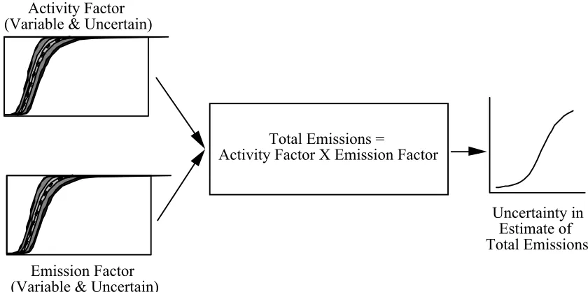
emissions-generating activity, therefore, a general emission inventory model, which can cover different emission sources, can be described as
E = A×EF (2-1) Where,
E = emissions (e.g., lb of NOx as NO2)
A = activity factor (e.g., tons of coal burned), and
EF = emission factor (e.g., lb of NOx as NO2 per ton of coal burned). In most cases, the emission factor and activity factor are often the outputs of other models describing emission factor or activity factors. For example, for a power plant unit, the activity factor is the product of the unit heat rate (BTU of fuel input required to produce one kWh of electricity), unit capacity factor (average capacity utilization for a given time), and unit capacity (MW). For highway vehicles emission sources, emission factor depends on mileage, deterioration rate, temperature, Reid vapor pressure and other parameters. A known model to describe the highway vehicle emission factors is
MOBILEx
categories. In general, if available, a known emission inventory model or an emission inventory model recommended by EPA for the specific source categories is encouraged to use in developing a probabilistic emission inventory.
2.4 Numerical sampling techniques
In order to analyze variability and uncertainty in model input or output, a
probabilistic modeling environment is required. Various techniques have been proposed for performing variability and uncertainty analysis, for example, internal analysis,
analytic method, numerical approximation approximations such as Taylor series expansion, and numerical sampling methods. Based on the limits, robustness, and mathematical complexity of these methods, numerical sampling techniques are the most widely used since it is the most robust and least restrictive with respect to model design and model input specification. Two numerical sampling techniques, Monte Carlo Sampling and Latin Hypercube Sampling are presented in the next subsequent sections.
2.4.1 Monte Carlo Sampling
In Monte Carlo method, a probability distribution is specified for each model input. Each distribution can be represented as a cumulative distribution function (CDF). Numerical methods based upon the use of a pseudo random number generator (PRNG) are used to generate random values from the assigned probability distribution model. There are several approaches for generating random numbers, for example, the method of inversion, the method of convoluation, the method of the composition, and the
acceptance –rejection method (Law and Kelton,1991). Of these methods, conceptually the most straight-forward is based upon the use of an inverse CDF. To generate a random number from a specified probability distribution model, first a pseudo random random number is generated from a uniform distribution over the range of zero to 1. The random number is then used as an estimate of cumulative probability as an input to the inverse CDF for the assigned probability distribution model. The output of the inverse CDF is a numerical value of the random variable of interest. This process is repeated n times, where n is the desired simulation sample size, to produce many estimates of a model input. This process is also conducted simultaneously, with different random values from the PRNG, for each of many probabilistic inputs to a model. The random values for each model input are used to calculate a model output values. The propagation of multiple model inputs through a model leads to a distribution of model output values that reflect the uncertainty or variability in the model inputs (Ang and Tang,1984). More information regarding random Monte Carlo method may be found in Morgan and
Henrion (1990), Cullen and Frey (1999) and others.
disadvantage is that it may be necessary to use large sample sizes to obtain smooth approximation of the CDF of a model output. Random Monte Carlo simulation is a desirable method when the objective is to simulate random sampling error. Other methods, such as Latin Hypercube Sampling, can produce smoother estimates of the empirical CDF of a model output with fewer samples than are needed using random Monte Carlo (Frey, et al., 1998b).
2.4.3 Latin Hypercube Sampling
As an alternative to random Monte Carlo sampling, Latin Hypercube Sampling (LHS), developed by McKay, Beckman, and Conover (1979), is a stratified sampling technique which can ensure that samples are taken from the entire range of a distribution. In LHS, the range of each input distribution is divided into n intervals of equal marginal probability. One value of the random variable is selected from each interval. The sample taken from each interval may be selected at random from within the interval, or from the median of the interval. The former is referred to as random LHS while the later is called median LHS. In both median and random LHS, the n values from each distribution are randomly paired with values generated for other model inputs. The stratification of the input distributions into n equal probability intervals ensures that samples are taken from the entire range of the distributions even with a relatively small sample size compared to random Monte Carlo sampling.
However, for some applications, LHS is a more precise numerical simulation method than random Monte Carlo for a given simulation sample size.
2.5 Visualization of Datasets Using Empirical Distributions
Some of the key purposes of visualizing data sets include: (1) evaluation of the central tendency and dispersion of the data; (2) visual inspection of the shape of the empirical distribution of the data as a potential aid in selecting parametric probability distribution models to fit to the data; and (3) identification of possible anomalies in the data set (e.g., outliers). Specific techniques for evaluating and visualizing data include calculation of summary statistics, and plotting a data set as an empirical Cumulative Distribution Function (CDF).
Three key characteristics of a CDF are its central tendency, dispersion, and shape. There are several measures of central tendency, which include the mean, median, and mode. The dispersion, or the spread, of a distribution is measured by the standard deviation or the variance of the distribution. The relative standard deviation (RSD), also known as the coefficient of variation (CV), is the standard deviation divided by the mean. For a non-zero mean, the CV provides a normalized indication of the dispersion of data values, with a large CV indicating relatively large variability in the data set. The shape of the distribution is reflected by quantities such as skewness and kurtosis. The skewness is the asymmetric of a distribution, and the kurtosis refers to the peakedness of a
distribution. These statistics can be used to aid in the selection of a parametric probability distribution model to fit to the data (Cullen and Frey, 1999).
provide a relationship between fractiles and quantiles. A fractile is the fraction of values that are less than or equal to a specific value of a random variable. Fractiles expressed on a percentage basis are referred to as percentiles. A quantile is the value of a random variable associated with a given fractile (Frey, Bharvirkar and Zheng, 1999). For
example, the range of data values enclosed by the 0.025 and 0.975 fractiles (2.5 and 97.5 percentiles) is often of particular interest, since this provides an indication of the
dispersion of a distribution as reflected by the 95 percent probability range of values. An example of a CDF is illustrated in Figure 2-1
Empirical estimation of a fractile from data requires rank ordering of the data. There are several possible methods for estimating the percentile of an empirically observed data point.
These methods are referred to as “plotting positions.” The plotting position is an estimate of the cumulative probability of a data point. As described by Cullen and Frey (1999), Harter (1984) provides an overview of the various types of plotting positions.
95 Percent Probability Range
200 300 400 500 600 700 800
NOx Emission Factor (Gram/ GJ Fuel Input) 0.0
0.2 0.4 0.6 0.8 1.0
Cumulative Probability