Design and Analysis of a Double Spiral
Counter Flow Heat Exchanger Using CFD
Kulkarni Pavan Venkatesh1, Prabhanjan Mishra1, Krishna Kumar1 , Ajay Krishna T M2, Sreenivas H T2
U.G. Student, Department of Mechanical Engineering, Vijaya Vittala Institute of Technology, Bangalore, Karnataka,
India1
Assistant Professor, Department of Mechanical Engineering, Vijaya Vittala Institute of Technology, Bangalore,
Karnataka, India2
ABSTRACT: Spiral flow heat exchangers are known as excellent heat exchanger because of far compact and high heat
transfer efficiency. SFHE is a unique design where it consists of single fluid as working fluid for heat exchange. Here heat transfer takes place between solid and fluid, and hence can be called as conjugate heat transfer. Heat transfer characteristics of SFHE are observed at various Reynolds number and base temperature. SFHE is designed and fabricated with new arrangement for measuring the heat transfer is employed for obtaining the experimental results. The concept of thermoelectric effect is used which is direct conversion of temperature difference to electric voltage, to measure temperature at various points in the heat exchanger. CAD model is developed and computations are performed using commercially available CFD package ANSYS-CFX for the same boundary conditions, input conditions as that considered for experimental purpose. Obtained CFD results are compared with that of experimental results for validation. It is observed that there is a good agreement between experimental and computational results. Optimization of the heat exchanger can be carried out using computational methods developed in this work for better performance.
KEYWORDS: Spiral Flow Heat Exchanger, Thermoelectric effect, Fabrication, ANSYS-CFX, Validation.
I. INTRODUCTION
of the unit and flows towards the periphery. The other fluid (cold fluid) enters the unit at the periphery and moves towards the centre. The channels are curved and have a uniform cross section, which creates “spiralling” motion within the fluid [5]. The fluid is fully turbulent at much lower velocity than straight tube heat exchangers, and fluid travels at constant velocity throughout the whole unit. Spiral tube heat exchanger consists of number of spirals attached to the header.
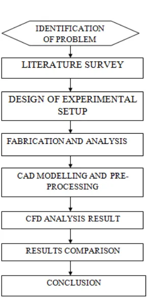
II.METHODOLOGY
Figure 1: Flowchart of the methodology
DESIGN OF EXPERIMENTAL SETUP
Figure 2: Design of the spiral flow heat exchanger
A spiral strip is used as a passage for the fluid flow and is constructed on the target plate having cross section area of 145 mm X 150 mm and thickness 3 mm, here we have used the spiral strip for our convenience, which is of thickness 3 mm, height 12 mm and passage 12 mm as shown in Fig 2. In this way, a square passage of flow of 12 X 12 sq. mm is obtained.
is 1/30th that of copper. Also the melting point is 1357.77 K and the maximum temperature to be carried out during the experiment is 373K.
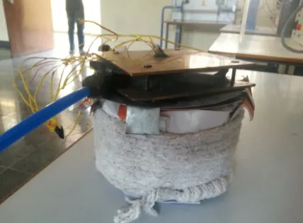
FABRICATION
The spiral coil is fabricated on the iso-thermal base plate. The fabrication is carried out by brazing process. Brazing is a metal-joining process whereby a filler metal is heated above melting point and distributed between two or more close-fitting parts by capillary action. The filler metal is brought slightly above its melting temperature while protected by a suitable atmosphere, usually a flux. It then flows over the base metal and is then cooled to join the work pieces together. It is similar to soldering, except the temperatures used to melt the filler metal are higher for brazing. Copper is brazed because it cannot be welded. This is because the temperature obtained during welding is high and almost equal to the melting point of copper. Hence, to avoid it brazing is done. The other base plate is fitted above the spiral coil using nuts and bolts with a rubber pad in between. The rubber acts as a means of insulator and means to avoid leakage. Even after completing the entire fabrication of SFHE, leakage was found at some places. The leakage is prevented by applying M-seal, which is combination of a resin base and hardener. Pipes of 10 mm are fitted at inlet and outlet for passage of water. Thermocouples are installed at following places: Three thermocouples in the central region, one at inlet, one at outlet and the last one immersed in the heat bath. The thermocouple wires are drawn out of the setup from the centre by drilling hole. The thermocouple wires are soldered at the channel-selector. Fig 3 shows a view of completely assembled SFHE. The base wound with asbestos and heat exchanger placed above it.
Figure 3: Final setup of the spiral flow heat exchanger
III.COMPUTATIONALAPPROACH
Fluid dynamics deals with the dynamic behaviour of fluids and its mathematical interpretation is called as Computational Fluid Dynamics. Fluid dynamics is governed by sets of partial differential equations, which in most cases are difficult or rather impossible to obtain analytical solution. CFD is a computational technology that enables the study of dynamics of things that flow.
Figure 4: Points & Curves used to develop CAD model
Figure 5: Base plate, Adiabatic strip & flow domain of the spiral flow heat exchanger
CAD modelling
CAD modelling is performed using ICEM CFD application. Tetra elements is used as it is most suitable for complex geometries and offers several benefits like rapid model setup, no surface mesh necessary, control over element size inside a volume and mesh independent of underlying surface topology. ANSYS-CFX package is used to perform analysis which uses RANS approach to solve the physical problem. CFD-POST is used to read the results in the form of Vector plots, contour plots and Particle tracking.
IV.RESULTS&COMPARISON
In this section results from experiment and computations are presented and compared. Results are obtained for base temperature of 100 ͦ C (373 K) and for various mass flow rates. Thermocouples were used to measure temperature in terms of milli Volts and were read in temperature using calibration graph of thermocouple wire. Computation results are obtained using ANSYS – CFD Post. Plots are plotted for parameters like temperature, pressure and velocity which help in evaluating the performance of the double spiral counter flow heat exchanger.
The variation in the experimental values may be caused due to many factors. Some of them are: fabrication errors, leakage of water, uneven base heating etc. It can also be viewed in the profiles that the temperature of the base plate decreases as the mass flow rate is increased. This shows that the heat transfer has increased due to increase in mass flow rate. Also, in pressure profile it is seen that the pressure at inlet is more and at outlet is less comparatively. This is because of the increase in velocity. In velocity profile, it can be seen that the velocity increases with increase in mass flow rate. This is mainly due to two reasons: Due to turbulence created in the centre of the setup and other reason is due to centrifugal force created as the fluid circulates in circular motion. In vector plot, we can see exactly where the turbulence is created. Turbulence is created when the vectors of the fluid start to cross each other’s path. So it is seen in the central part of the SFHE.
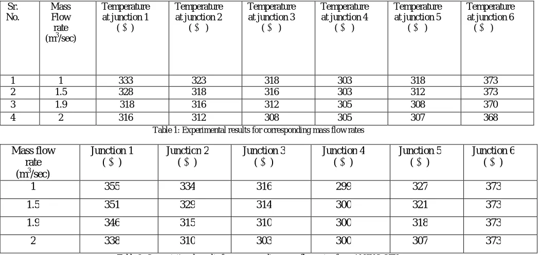
The thermocouples are placed at six places in the heat exchanger. Those are as follows:
Junction 1 – Base plate at the centre of the heat exchanger Junction 4 – Inlet of the heat exchanger Junction 2 – Wall of the spiral passage at the centre Junction 5 – Outlet of the heat exchanger Junction 3 – Top of the spiral wall at the centre Junction 6 – Hot water bath
The experimental results are shown in the table below.
Sr. No.
Mass Flow rate (m3/sec)
Temperature at junction 1
( ͦ K)
Temperature at junction 2
( ͦ K )
Temperature at junction 3
( ͦ K )
Temperature at junction 4
( ͦ K )
Temperature at junction 5
( ͦ K )
Temperature at junction 6 ( ͦ K )
1 1 333 323 318 303 318 373
2 1.5 328 318 316 303 312 373
3 1.9 318 316 312 305 308 370
4 2 316 312 308 305 307 368
Table 1: Experimental results for corresponding mass flow rates
Mass flow rate (m3/sec)
Junction 1 ( ͦ K)
Junction 2 ( ͦ K)
Junction 3 ( ͦ K)
Junction 4 ( ͦ K)
Junction 5 ( ͦ K)
Junction 6 ( ͦ K)
1 355 334 316 299 327 373
1.5 351 329 314 300 321 373
1.9 346 315 310 300 318 373
2 338 310 303 300 307 373
The profiles obtained in ANSYS Post processor are shown below:
The temperature on the wall gradually decreases due to convection occurring between the wall and the fluid. Finally, it can be observed that the temperature on the adiabatic wall is minimum. This is because of the cooling of water. From the pressure profiles it is seen that the pressure is high at the inlet and low at the outlet of the SFHE. Hence, the velocity is more at outlet.
From the velocity profiles it is seen that velocity is maximum at the centre of the SFHE. This is because turbulence is created at the centre due to sudden change in direction. It can also be seen that the velocity is more towards outer wall. This is because; the centrifugal force created due to circular movement of the water pushes the water towards the outer wall.
COMPARISON
It can also be viewed in the profiles that the temperature of the base plate decreases as the mass flow rate is increased. This shows that the heat transfer has increased due to increase in mass flow rate. Also, in pressure profile it is seen that the pressure at inlet is more and at outlet is less comparatively. This is because of the increase in velocity. In velocity profile, it can be seen that the velocity increases with increase in mass flow rate. This is
Figure 7: Temperature profile for 1m3/sec Figure 8: Velocity streamline for 1m3/sec Figure 9: Pressure profile for 1m3/sec
Figure 10: Temperature profile for 1.5m3/sec Figure 11: Velocity streamline for 1.5m3/sec Figure 12: Pressure profile for 1.5m3/sec
Figure 13: Temperature profile for 1.9m3/sec Figure 14: Velocity streamline for 1.9m3/sec Figure 15: Pressure profile for 1.9m3/sec
mainly due to two reasons: Due to turbulence created in the centre of the setup and other reason is due to centrifugal force created as the fluid circulates in circular motion.
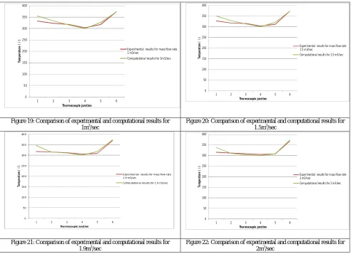
The comparison of experimental and computational results can be viewed in the graphs below:
0 50 100 150 200 250 300 350 400
1 2 3 4 5 6
Te m p e ra tu re ( ͦK ) Thermocouple junction
Experimental results for mass flow rate 1 m3/sec
Computational results for 1m3/sec
0 50 100 150 200 250 300 350 400
1 2 3 4 5 6
Te m p e ra tu re ( ͦK) Thermocouple junction
Experimental results for mass flow rate 1.5 m3/sec
Computational results for 1.5 m3/sec
Figure 19: Comparison of experimental and computational results for 1m3/sec
Figure 20: Comparison of experimental and computational results for 1.5m3/sec
0 50 100 150 200 250 300 350 400
1 2 3 4 5 6
Te m p e rat u re ( ͦK)
Thermocouple junction
Experimental results for mass flow rate 1.9 m3/sec
Computational results for 1.9 m3/sec
0 50 100 150 200 250 300 350 400
1 2 3 4 5 6
Te m p e ra tu re ( ͦK ) Thermocouple junction
Experimental results for mass flow rate 2 m3/sec
Computational results for 2 m3/sec
Figure 21: Comparison of experimental and computational results for 1.9m3/sec
Figure 22: Comparison of experimental and computational results for 2m3/sec
V. CONCLUSION
For steady state analysis, the pressure drop for calorimeter along the length of the flow is found to be uniform except at the mid length and found to be increasing with the mass flow rate. At the centre of the plate there is sharp decline in pressure due to change in the cross sectional area of flow. The pressure recovery takes place in a short distance.
It is observed that temperature of water gradually increased along the flow length because it picks up heat during the course of the flow. There is a clear evidence of the heat transfer cross the vertical strip separating the adjacent counter flow hot and cold steams. For constant inlet and base temperatures, the outlet temperature of the water decreases with mass flow rate. Velocity suddenly increases at mid length due to change in cross section area of SFHE, velocity recovers in a short distance in the downstream and remains almost constant till the outlet. There is no evidence of the influence of the base temperature on the velocity distribution.
REFERENCES [1] P.E. Minton, “Designing Spiral-Plate Heat exchangers”, Union Carbide Corp.
[2] Jay J. Bhavsar, V K. Matawala, S. Dixit, “Design and Experimental Analysis of Spiral tube heat exchanger”, Shri S’ AD Vidhya Mandal Institute of Technology, Bharuch.
[3] Martin Martinez Garcia & Miguel Angel Moreles, “A Numerical Method for rating Thermal performance in Spiral Heat exchangers”, University of Guanajuato..
[4] M. Picon Nunez, L. Canizalez Davalos and A. Morales Fuentes, “Alternative design approach for spiral plate heat exchangers”, Institute of Scientific research, University of Guanajuato.
[5] Achmad Nursyamsu, Dr. Ir. Ahmad Indra S (2007) “Analysis of fluid flow in pipes with spiral on the variation pitch computational fluid dynamics using (CFD)”: Undergraduate Program, Gunadarma University.
[6] Santosh M. Bagewadi “Cfd Analysis Of Double Spiral Counter Flow Calorimeter In Impinging Flame Jet”.
[7] Dhanawade Hanamant S, K. N. Vijaykumar, Dhanawade Kavita: “Natural Convection Heat Transfer Flow Visualization Of Perforated Fin Arrays By CFD Simulation”.
[8] M. P. Nueza & G.T. Polley & L. C.Davalos & G. M. Rodriguez, “Design Approach For Spiral Heat Exchangers”, Institution of Chemical Engineers, Vol. 85, PP–322–327, 2007.
[9] Minton, H. “Designing Spiral Heat Exchangers”, Chemical engineering, May, PP–103–112, 1990. [10] Holger, M, “Heat exchangers”, Hemisphere Publishing Corporation, London, 1992.
[11] Jayakumara J.S, Mahajania S.M, Mandala J.C, Vijayanb P.K, “Experimental and CFD estimation of heat transfer in helically coiled heat exchangers”, 1997.
[12] Rogers, G.F.C. and Mayhew, Y.R., (1964) ”Heat transfer and pressure drop in helically coiled tubes with turbulent flow”. International Journal Heat Mass Transfer.