Surface Finish and Form Fidelity in Diamond Turning

(1)

ABSTRACT

LAMONDS, DONALD LUCAS. Surface Finish and Form fidelity in Diamond Turning. (Under the direction of Thomas A. Dow.)

Fabrication of imaging systems requires nanometer precision of the optical form and

micrometer precision in the position of that surface relative to the imaging system. To

gain experience with production of optical systems and prepare for non-rotationally

symmetric systems, a two-mirror axisymmetric Richey-Chrétien telescope was fabricated

with a diamond turning machine; based on the measurements of the telescope, further

modeling and experimentation was done to verify the form-error capability of the

machine and surface finish with machine vibration.

Optical flats were fabricated in a fashion that revealed the error motions of the diamond

turning machine. Squareness between the axes was found as the dominating error and

compensation was first attempted by setting the tool path equal to the inverse of the error.

Automatic error correction routines written prior to this work were re-activated and the

correct squareness compensation was input. Several optical flats were fabricated using

different tool locations on the DTM and all measurements showed traces at !/4. A sphere

was then fabricated that had less the !/4 form error with optical power (spherical radius

error) removed and the spherical radius was within 6 !m of the target. When observing

the conditions described in this work, optical surfaces can repeatedly be fabricated with

(2)

Initial surface finish tests were conducted at machining rates where the parabolic

approximation should accurately predict peak-to-valley surface finish. These tests were

designed to check for surface finish dependence on cutting depth, surface speed, and

cross-feed rate. Results indicated that finish was dependant on cross feed-rate but that

there were other factors causing increased roughness. Further examination of the results

showed that machine vibration and minimum chip thickness (a variable dependant on tool

edge sharpness) were adding to roughness. A model was created to predict surface

roughness influenced by machine vibration and experiments to prove the model used a

freshly sharpened tool. The model results predicted that surface finish can be improve

beyond the vibration amplitude of the machine as did the experimental results. The

model was expanded to further improve the finish quality by dithering the tool in the

cross-feed direction such that diffraction patterns from diamond turned cusps were

smooth rather than periodic. Scatter measurements were taken from the workpiece used

in machine tests vibrations tests and it was found that the desired effects of tool dithering

were present in the lower, optical surface quality feed-rates (1-2 !m/rev). This result

(3)

Surface Finish and Form Fidelity in Diamond Turning

by

Donald Lucas Lamonds

A thesis submitted to the Graduate Faculty of North Carolina State University

In partial fulfillment of the requirements for the Degree of

Master of Science

Mechanical and Aerospace Engineering

Raleigh, NC

2008

APPROVED BY:

____________________________ ____________________________ Gregory D. Buckner Ronald O. Scattergood

___________________________ Thomas A. Dow

(4)

DEDICATION

To Laura, whose patience was greater than any and whose love I did, and will eternally

(5)

BIOGRAPHY

D. Lucas Lamonds was born in Winston-Salem, NC and was raised in Mocksville, NC.

He graduated from Davie County High School in the spring of 1997 and attended North

Carolina State University in the fall. While attending NC State, he had internships with

AMP, R.J. Reynolds machine shop and Getrag Gears LLC. Lucas graduated from NC

State in 2002 with a Bachelor of Science in Mechanical Engineering. After graduation,

he then began employment with Getrag Gears LLC in Charleston SC as a quality and

manufacturing engineer. In January 2005, Lucas returned to NC State University to start

(6)

ACKNOWLEDGMENTS

I would like to thank everyone who help me along the way. Acknowledgments

• Dr Dow, For his direction, drive, knowledge and scientific mentality.

• Ken Garrard and Alex Sohn, For their proficiency all the equipment, sharing their

past PEC experiences and for fascinating discussions.

• Nadim Wanna and Rob Woodside, For their camaraderie in classes, at the PEC

and away from NC State.

• The students at the PEC, Dave, Kara, Tim, Chen, For Friday lunches and relieving

conversations.

• Laura, For her unwavering support.

(7)

LIST OF FIGURES

FIGURE 2-1: ROUGH MACHINED COMPONENTS OF THE TWO-MIRROR TELESCOPE... 7 FIGURE 2-2:THE OPTICAL PATH OF THE RICHEY-CHRÉTIEN TELESCOPE WITH OPTICAL ELEMENTS AND

SPECIFICATIONS. INCIDENT LIGHT FROM THE OBJECT (INFINITE CONJUGATES) ENTERS FROM THE LEFT AND THE IMAGE IS FORMED ON THE RIGHT. PATH GENERATED WITH OSLO-EDU® FROM LAMBDA

RESEARCH CORPORATION... 8

FIGURE 2-3: CROSS SECTION OF TELESCOPE COMPONENTS WITH DARK LINES INDICATING SURFACES THAT WERE DIAMOND TURNED. DASHED LINE SHOWS THE COMMON AXIS OF SYMMETRY/ROTATION... 9

FIGURE 2-4: FINAL ASSEMBLED OPTICAL SYSTEM. ...10 FIGURE 2-5: RANK-PNEUMO ASG-2500 DIAMOND TURNING MACHINE...15 FIGURE 2-6: FABRICATION OF RICHEY-CHRÉTIEN TELESCOPE COMPONENTS ON THE ASG-2500 DTM WITH

A DASHED LINE TO SHOW THE COLLINEAR OPTICAL, TUBE AND SPINDLE AXES...16 FIGURE 2-7:TOOL LAYOUT ON THE DTM ILLUSTRATING THE RELATIVE LOCATION OF THE TWO TOOLS AND

THE 10X TELESCOPE (BLACK CYLINDER ON RIGHT OF PHOTO). ...17 FIGURE 2-8: OGIVE ERROR CAUSED BY TOOL GOING PAST SPINDLE CENTER IN X DIRECTION...18

FIGURE 2-9: CENTERING PLUG MOUNTED IN HOLDER, WHICH IS VACUUMED TO CHUCK...20 FIGURE 2-10: HEIGHT GAGE USED TO SET THE DIAMOND TOOL HEIGHT (Y-DIRECTION) AT SETUP. THE

DIAMOND IS RAISED INTO GAGE TIP BY TURNING THE KNOB ON THE TOOL POST...21

FIGURE 2-11: TWO DIAMOND TURNED GROOVES CUT IN THE END OF A CENTERING PLUG...22

FIGURE 2-12: SCREEN CAPTURE OF THE NEW VIEW MEASUREMENT SHOWING A CENTERING ERROR IN THE VERTICAL DIRECTION (Y). THE CYLINDRICAL SHAPE INDICATES THE TOOL WAS LOW OF CENTERLINE.

...24

(12)

FIGURE 2-14: SPIRAL AT CENTER OF WORKPIECE WHERE RADIAL LINES CREATED BY SPINDLE AIR-BEARING PADS ARE VISIBLE. DARK LINES HIGHLIGHT TWO OPPOSING MARKS THAT, WITH COUNTER CLOCKWISE SPINDLE ROTATION, INDICATE TOOL WAS LOW. ...26 FIGURE 2-15: CROSS SECTIONAL ERROR SHAPES FOR A CENTERING PLUG SPHERE IN THE HORIZONTAL

DIRECTION (X)...27 FIGURE 2-16:SCREEN SHOT OF GPI OUTPUT SHOWING A CENTERING ERROR IN THE HORIZONTAL DIRECTION

(X) WHERE THE TOOL WAS LONG OF CENTER. TRACE SHAPE SEEN IN FIGURE 2-15A. ...28 FIGURE 2-17: ILLUSTRATION OF SURFACE NORMAL VECTORS AND TOOL OFFSET TO FORM DISCRETE TOOL

PATH. DESIRED SURFACE IS A CONTINUOUS FUNCTION AND THE NORMAL VECTOR LENGTH IS EQUAL TO THE TOOL RADIUS. ...32

FIGURE 2-18: CROSS-SECTION OF DESIRED PRIMARY OPTICAL SURFACE (SOLID LINE) AND TOOL RADIUS COMPENSATED MACHINING PATH (DASHED LINE) WITH CIRCLES REPRESENTING THE TOOL RADIUS. TO SCALE. ...34 FIGURE 2-19: PRIMARY (UPPER) AND SECONDARY (LOWER) MIRROR MOTION PLOTS DRAWN BY K.

GARRARD. THE CIRCLES (O) IDENTIFY THE UNCOMPENSATED TOOL PATH WHILE LINES PASSING THROUGH THE CIRCLES LABELED HYPERBOLA ARE THE SURFACE AS SPECIFIED BY THE OPTICAL DESIGN. LINES LABELED TOOL PATH ARE THE TOOL RADIUS COMPENSATED PATH. ...35 FIGURE 2-20: PRIMARY (LEFT) AND SECONDARY (RIGHT) MIRROR MOTION PATH ERROR FILTERED WITH 100

POINT MOVING AVERAGE BY K GARRARD. THIS SHOWS THE DIFFERENCE BETWEEN COMMANDED PATH AND THE ACTUAL PATH AS MEASURED BY THE LASER INTERFEROMETER FEEDBACK OF THE ASG-2500 CONTROL SYSTEM. ...37 FIGURE 2-21: VACUUM CHUCK FLATNESS (LEFT) AND RUNOUT (RIGHT) AS MEASURED FOR TWO MIRROR

(13)

FIGURE 2-25: SECONDARY MIRROR AND SUPPORT STRUCTURE AFTER DIAMOND TURNING. ...46

FIGURE 2-26:SECONDARY ON VACUUM CHUCK WITH VACUUM PLATE. CRITICAL FIDUCIAL SURFACES ARE IN BOLD...47

FIGURE 2-27: DIGITIZED SECONDARY BACK. OUTER RING REPRESENTS THE BACK OF THE FIDUCIAL STEP. CENTER CLUSTER IS THE MIRROR BACK. POINTS ALONG THE THREE LEGS SHOWN FOR CLARITY. ...49

FIGURE 2-28: CROSS SECTION OF SECONDARY MIRROR STRUCTURE ILLUSTRATING THE 20 !M OFFSET BETWEEN THE MIRROR BACK AND THE OUTER RING. ...49

FIGURE 2-29: TUBE CROSS SECTION SHOWING RADIAL SEATING SURFACES AND AXIAL SEATING SURFACES. 52 FIGURE 2-30: MACHINING THE TUBE WITH DTM. ...53

FIGURE 3-1: GEOMETRICAL LAYOUT OF THE ASG-2500 SLIDES WITH DIRECTIONS LABELED. Z INTERFEROMETER IS NEXT TO THE SPINDLE AND X INTERFEROMETER IS RIGHT OF TOOL HOLDER; FOR CLARITY, THE INTERFEROMETER MOUNTING PLATES AND OIL GUARDS ARE NOT SHOWN. ...62

FIGURE 3-2:X AND Z-AXIS STRAIGHTNESS (NOTE SCALE DIFFERENCE) WITH (SOLID LINE) AND WITHOUT (DASHED LINE) COMPENSATION FROM THE ORTHOGONAL SLIDE. [4] ...63

FIGURE 3-3: TOOL PATH AND OIL SPRAY FOR DIAMOND TURNED FLATS EXPERIMENT. TO SCALE...65

FIGURE 3-4:Z-AXIS YAW OVER FULL 150 MM RANGE IS 1.6 ARCSEC. ...67

FIGURE 3-5: ZYGO GPI HPXR FORM MEASURING INTERFEROMETER WITH METROPRO SOFTWARE. ...69

FIGURE 3-6: EXAMPLE TRACE (#13 FROM TABLE 3-1) OF 6061 T-6 FLAT MACHINED ON THE DTM WITH YAW CORRECTION OF 0.7 ARC-SECONDS. ...73

FIGURE 3-7: SLOW VELOCITY X-AXIS MOVE. LINEAR CURVE FIT SLOPE = 0.0165 MM/S. ...74

FIGURE 3-8: FINAL MANUALLY CORRECTED SQUARENESS ERROR SHOWING CONVEX SHAPE...74

FIGURE 3-9: COMPARISON OF 6061 WORKPIECE AND THE FINAL SHAPE OF THE FLAT TESTS. ...76

FIGURE 3-10: 6061-T6 WORKPIECE WITH 150 MM OPTICAL SURFACE DIAMETER. UPPER LEFT CORNER TRIMMED OUT BECAUSE IT WAS NOT MACHINED DURING THIS PASS...78

(14)

FIGURE 3-12: ZYGO GPI FORM MEASURING LASER INTERFEROMETER STAGE FITTED WITH A LENGTH

MEASURING INTERFEROMETER. ...81

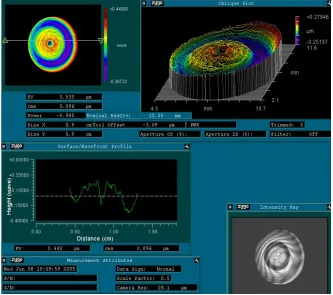
FIGURE 3-13: INTERFEROGRAM SEEN WHEN THE GPI FOCUS IS ALIGNED WITH THE APEX OF THE SPHERE USING THE “CAT’S EYE” TECHNIQUE. POWER IS ALMOST ZERO (0.037 != 23 NM RADIUS).

HORIZONTAL AND VERTICAL SCALES SHOULD BE IGNORED BECAUSE THIS MEASUREMENT IS AN INTERFEROGRAM OF A SPOT (APEX OF THE SPHERE). ...82 FIGURE 3-14: SPHERE MEASUREMENT WITH POWER REMOVED. PV ERROR WAS 150 NM OR "/4. ...83 FIGURE 4-1:TRANSITION FROM 2 !M CUTTING DEPTH TO 1 !M AT 37.7 !M/REV FEED RATE, AND 1.1 M/S

SURFACE SPEED IN ELECTROPLATED COPPER WITH A 0.750 MM RADIUS TOOL. CROSS FEED DIRECTION IS FROM LEFT TO RIGHT IN THIS AND ALL OTHER SURFACE PROFILES IN THIS SECTION. ...89 FIGURE 4-2: SECOND-ORDER EFFECT OF MINIMUM CHIP THICKNESS CAUSED BY A WORN TOOL WITH A LARGE EDGE RADIUS [13]...91 FIGURE 4-3: RAKE FACE AREA ENCLOSED BY THE PREVIOUS PASS, TOOL EDGE AND UNCUT SURFACE. THE

RATIO OF LENGTH TO HEIGHT IN THIS DRAWING WAS SET TO RESEMBLE FIGURE 4-1 AT

APPROXIMATELY 150:1. ...92

FIGURE 4-4:DIAMOND TURNING MACHINE WITH FTS FOR INSTANT DEPTH OF CUT CHANGE...94 FIGURE 4-5: OPEN LOOP RESPONSE OF FTS WITH 40 MM PZT STACK...96

FIGURE 4-6: 1 !M CUTTING DEPTH CHANGE COMMAND AT A CIRCUMFERENCE OF 125MM. RISE TIME IS 5.3 MS...97 FIGURE 4-7: EXAMPLE OF TOOL PATH WITH INSTANT DEPTH OF CUT CHANGES. THE ORIGINAL SURFACE IS

SEEN AT FAR LEFT AND RIGHT OF THE PROFILE. THE DEEPEST CUT IS ON THE LEFT AND WAS

(15)

FIGURE 4-10: ACTUAL AND THEORETICAL SURFACE ROUGHNESS VS. DEPTH OF CUT FOR TESTS 1-3. THREE POINTS AT EACH CUTTING DEPTH FROM TESTS 1-3. F = 37.7 !M/REV. ...104

FIGURE 4-11:ACTUAL AND THEORETICAL PV SURFACE ROUGHNESS VS. FEED RATE FOR TESTS 1-7 IN TABLE

4-1. ...105

FIGURE 4-12: ACTUAL AND THEORETICAL RMS SURFACE ROUGHNESS VS. FEED RATE FOR TESTS 1-7 IN

TABLE 4-1. ...106

FIGURE 4-13: 1 !M DEPTH OF CUT CHANGE FOR 5.33 !M/REV FEED RATE...107 FIGURE 4-14: SURFACE PROFILE FROM A 37.7 !M/REV FEED RATE (TEST 1) SHOWING SEVERAL CUSPS WITH

THE LAST GROOVE CUT AT THAT DEPTH BEFORE THE FTS STEPPED THE TOOL UP COMPARED TO THE THEORETICAL PROFILE (SMOOTH LINE). ...109

FIGURE 4-15:SURFACE PROFILE FROM A 5.33 !M/REV FEED RATE (TEST 4D) SHOWING SEVERAL CUSPS AND THE LAST GROOVE CUT AT THAT DEPTH BEFORE THE FTS STEPPED THE TOOL UP COMPARED TO THE THEORETICAL PROFILE (SMOOTH LINE). THIS GRAPH HAS 10X THE VERTICAL MAGNIFICATION OF

FIGURE 4-14...109

FIGURE 4-16: 37.7 !M/REV FEED RATE (TEST 1) ZOOMED TO SHOW ONLY A FEW CUSPS AND COMPARED TO THEORETICAL (SMOOTH LINE). FEED DIRECTION LEFT TO RIGHT...111

FIGURE 4-17:11.9 !M/REV FEED RATE (TEST 4C) WITH CUTTING DEPTH CHANGE COMPARED TO

THEORETICAL PROFILE (SMOOTH LINE). ASYNCHRONOUS VIBRATION CAUSED VALLEY-TO-VALLEY VARIATION OF 22 NM. FEED DIRECTION LEFT TO RIGHT...111 FIGURE 4-18: ORIENTATION OF UP FEED TRACE IN FIGURE 4-19. ...112 FIGURE 4-19: TRACE MEASUREMENT IN THE CUTTING DIRECTION (UP-FEED). TOOL MOVED FROM THE LEFT

OF THE TRACE TO THE RIGHT. TEST 3: F = 37.7 !M/REV, CUTTING DEPTH = 5 !M, SURFACE SPEED =

0.085 M/MIN. FEATURE SPACING IS 1.5 !M AS SEEN IN AUTOCOVARIANCE PLOT MENU XPOS. ...113 FIGURE 4-20: DIAMOND-TURNED CUSPS FORMING SPIRAL FOUND AT CENTER OF WORKPIECE AFTER LAST

TOOL CENTERING ADJUSTMENT. ...120 FIGURE 4-21: CENTER FEATURE FOUND IN FIGURE 4-23 WITH A SPIRAL TRACE ALIGNED TO THE GROOVE

(16)

FIGURE 4-22: 3D PLOT OF INTERPOLATED POINTS FROM THE SPIRAL TRACE IN FIGURE 4-24...121 FIGURE 4-23: FREQUENCY RESPONSE OF SPIRAL PROFILE SEEN IN FIGURE 4-24...122

FIGURE 4-24:X AND " VECTORS OF TOOL CENTER SHOWING MODEL COORDINATE SYSTEM WITH

RELATIONSHIP TO WORKPIECE AND ROTATION CENTERLINE. ...126 FIGURE 4-25: CERTAIN POINTS FROM MULTIPLE TOOL CUPS (CIRCLES), AT VARYING DEPTHS DUE TO

VIBRATION, PRODUCE A FINISHED SURFACE CONTOUR (LINE)...129 FIGURE 4-26: CONSECUTIVE SURFACE CONTOURS IN THE CROSS-FEED DIRECTION (X) WERE STACKED IN THE

UP-FEED DIRECTION (Y) INTO A 3-D SURFACE...130

FIGURE 4-27: AT FINE CROSS-FEED RATES, SOME PASSES OF THE TOOL (+) ARE NOT REPRESENTED IN THE FINISHED SURFACE. THIS PRODUCES A BETTER FINISH THAN WOULD BE EXPECTED FROM THE RMS OF THE VIBRATION ALONE. ...131

FIGURE 4-28: AS THEORETICAL SURFACE FINISH DECREASES, THE EFFECTS OF MACHINE VIBRATION ON SURFACE FINISHED ARE REDUCED. VIBRATION PV = 22 NM AND RMS = 7.7 NM...132 FIGURE 4-29: TYPICAL SURFACE PROFILE MEASUREMENT ILLUSTRATING THE DEPTH CHANGE AS A RESULT

OF VIBRATION WITH LARGE FEED RATE OF 11.3 !M/REV. THEORETICAL PV = 33 AND THEORETICAL

RMS = 10 NM DRAWN WITH BOLD LINE...134 FIGURE 4-30: TYPICAL MEASUREMENTS RESULT IN OBLIQUE PLOT FORM. THIS IS THE SAME SURFACE SHOWN

IN FIGURE 4-29. ...134

FIGURE 4-31: RESULTS FROM EXPERIMENTAL AND MODEL DATA WITH THRESHOLD OF RMS Z-AXIS

VIBRATION, A CURVE TO REPRESENT THE THEORETICAL PARABOLIC RMS SURFACE ROUGHNESS AND A DASHED LINE TO REPRESENT MODEL PREDICTION...136

FIGURE 4-32: MEASUREMENT OF 1.13 !M/REV CROSS-FEED WITH 3D PROFILE, CROSS-FEED TRACE,

(17)

FIGURE 4-34: MEASUREMENT OF 1.13 !M/REV CROSS-FEED WITH 3D PROFILE, CROSS-FEED TRACE,

AUTOCOVARIANCE OF TRACE, AND PSD OF TRACE. LITTLE INDICATION OF CROSS-FEED IS SEEN BUT LARGER SPACING IS SHOWN. ...140 FIGURE 4-35: MEASUREMENT OF 3.58 !M/REV CROSS-FEED WITH 3D PROFILE, CROSS-FEED TRACE,

AUTOCOVARIANCE OF TRACE, AND PSD OF TRACE. PSD SHOWS SMALL PEAK AT FEED RATE (3.58

!M/REV = 0.27 1/!M) ...141

FIGURE 4-36: PSD OF MODELED SURFACE PROFILE WITH 3.58 !M/REV. VIBRATION AMPLITUDE REDUCED TO

9 NM (FROM 11 NM) WHERE A PEAK AT 0.27 1/!M WAS EVIDENT. THIS MATCHES THE PSD IN FIGURE

4-35. ...142

FIGURE 4-37:MEASUREMENT OF 5.06 !M/REV CROSS-FEED WITH 3D PROFILE, CROSS-FEED TRACE,

AUTOCOVARIANCE OF TRACE, AND PSD OF TRACE. PSD HAS A PEAK AT THE FEED RATE (5.06 !M/REV

= 0.20 1/!M). ...143

FIGURE 4-38: PSD OF MODELED SURFACE PROFILE WITH 5.06 !M/REV. VIBRATION AMPLITUDE WAS REDUCED TO 9 NM (WAS 11 NM) WHERE A PEAK AT 0.20 1/!M WAS EVIDENT...144

FIGURE 4-39: DIFFRACTION PATTERN FROM A SINUSOIDAL SURFACE. ...147 FIGURE 4-40: SURFACE PROFILE OF PERFECT DIAMOND TURNED CUSPS. F = 5 !M/REV, R = 570 !M, PV =

5.4 NM AND RMS = 1.6 NM. ...151 FIGURE 4-41: AUTOCOVARIANCE FOR SURFACE IN FIGURE 4-40...152

FIGURE 4-42: LOG OF PSD NORMALIZED FOR THE MAXIMUM PEAK FROM AUTOCOVARIANCE IN 4-41. FIRST PEAK IS AT 0.2 FEATURES/!M OR 5 !M/FEATURE...152

FIGURE 4-43: SCATTER PATTERNS FOR VARIOUS SURFACE PROFILES. ...154 FIGURE 4-44: EXAMPLE OF DITHER CONCEPT (WITHOUT MACHINE VIBRATION DISTURBING THE CUSPS IN THE

Z-DIRECTION) SHOWING APEX OF TOOL (+) MOVED FROM REGULARLY SPACED INTERVALS (CROSS

-FEED) AND RESULTANT CONTOUR OF CIRCULAR CUSPS. A 570 !M NOSE RADIUS TOOL WAS USED WITH A 5 !M/REV CROSS FEED. PV = 10 NM AND RMS = 2.4 NM...156 FIGURE 4-45: SAMPLE 3D SURFACE PROFILE WITH CROSS FEED DITHERING (MOTION ALONG THE X-AXIS)

(18)

FIGURE 4-46: SURFACE PROFILE FOR AUTOCOVARIANCE SEEN IN FIGURE 4-47. F = 5 !M/REV AND R = 570

!M. ...160

FIGURE 4-47: AUTOCOVARIANCE OF THEORETICAL PROFILE IN FIGURE 4-43 WHERE F =5 !M/REV, R = 570

!M, PV =5.5 NM, RMS = 1.6 NM, G(0) = RMS2= 2.56 NM2...161

FIGURE 4-48:AUTOCOVARIANCE (DOTS), HILBERT TRANSFORM (SOLID) AND EXPONENTIAL DECAY FIT

(DASHED) OF FIGURE 4-47. ...163

FIGURE 4-50: DITHER EXAMPLES FOR THE 11.55 !M/REV FEED RATE. MACHINE VIBRATION IS INCLUDED (11

NM AMPLITUDE AT 63.6 HZ). ...164

FIGURE 4-51: Y-AXIS INTERCEPTS (B) VS DITHER AMPLITUDE WITH MACHINE VIBRATION PRESENT. LOWER VALUES OF B INDICATE LESS SURFACE AGREEMENT. SAME MODELED CUTTING CONDITIONS ARE SHOWN BELOW IN FIGURE 4-51...166

FIGURE 4-52:RMS SURFACE FINISH VS DITHER AMPLITUDE FOR THREE CROSS FEED RATES (UM/REV) WITH MACHINE VIBRATION PRESENT. SAME MODELED CUTTING CONDITIONS USED ABOVE IN FIGURE 4-50. ...166

FIGURE 4-53: SCATTER PATTERN MEASUREMENT SETUP. DASHED LINE SHOWS BEAM PATH. THE MIRRORED GLASS REFERENCE IS LYING BESIDE THE OPTICAL SETUP. THE FINAL FOLD MIRROR, PINHOLE

APERTURES AND THE DIAMOND TURNED SAMPLE ARE MOUNTED ON THE OPTICAL RAIL...169 FIGURE 4-54: ALTERNATE VIEW OF PAPER PINHOLE APERTURES. FROM FOREGROUND TO BACKGROUND:

FINAL FOLD MIRROR, FIRST APERTURE AND FINAL APERTURE. THE LARGE DOT ON THE FIRST APERTURE REPRESENTS A BEAM DIAMETER OF ABOUT 4 MM. ...170

(19)

LIST OF TABLES

TABLE 2-1: VICKERS HARDNESS VALUES FOR ROUGH MACHINED TELESCOPE COMPONENTS...13 TABLE 3-1: RESULTS OF 6061 T-6 ALUMINUM MACHINING TEST TO PRODUCE FLAT SPECIMENS. *FOR TESTS

15 & 16, THE AUTOMATIC MASK WAS SET TO 5% ID AND STILL USED 95% OD. ...71

TABLE 4-1: LAYOUT OF TESTS ON COPPER WORKPIECE. ...100 TABLE 4-2: ANGLES OF DIFFRACTION FOR FOUR DIFFRACTION ORDERS AND FOUR WAVELENGTHS OVER

VISIBLE (WHITE LIGHT) SPECTRUM. INCIDENT BEAM IS PARALLEL WITH THE SURFACE NORMAL (!I=

0º) AND THE SURFACE SPATIAL FREQUENCY IS 0.2 WAVES/!M (OR 5 !M SINUSOID WAVELENGTH)....149 TABLE 4-3: HILBERT TRANSFORMS []. ...162

(20)

1 INTRODUCTION

1.1 B

ACKGROUND

Diamond turned optics have been widely utilized in infrared and near-infrared imaging

systems. These systems were placed in military applications including missile defense

systems [9, 30]. They are typically rotationally symmetric and fabricated from an

aerospace material, such as 6061-T6 aluminum alloy and the surface is sometimes coated

with an impurity-free homogeneous (from the diamond tool perspective) material to

improve surface finish [9].

Future applications include three-mirror systems that utilize free-form optical surfaces

with no axis of rotation. Surfaces with no axis of rotation are currently being fabricated

with diamond turning machines [21]. The performance of systems designed with

free-from optics is often diffraction limited [28] and, according to the Rayleigh criterion, this

performance is maintained for up to a quarter-wave peak-to-valley deviation from the

designed wavefront [31]. Before fabrication of these non-rotationally symmetric optical

components is attempted, the ability to fabricate less complicated axisymmetric systems

with the Rayleigh criterion as a reference must be explored. Challenges in fabrication of

(21)

1.2 P

REVIOUS

R

ESEARCH

Single-point diamond turning machines commercially available in the late 1980s and

early 1990’s (like the Rank Pneumo ASG 2500) are typically equipped with oil

hydrostatic bearings, ball screw drives for axis actuation, air bearing spindles, and laser

interferometers for position feedback [9]. These machines are reported to create surface

finishes in 6061 aluminum of approximately 40 nm PV and 6-7 nm RMS [9]. This is

useful for the wavelengths in the near infrared spectrum and larger because these

wavelengths will scatter from diamond turned surfaces at large angles (incoherent scatter)

[16]. Newer machines with brushless DC linear motors for axis actuation and high-speed

spindles have been reported to produce smoother roughness on surfaces coated with a

single-phase material such as pure aluminum plating (Alumaplate®). Surface Roughness

approaching 1 nm RMS has been reported and these diamond turned surfaces are

reportedly adequate for use in the visible light spectrum. [6]

More recent research [19] has further explored the use of diamond turned 6061-T6

aluminum surfaces in white light applications. The optical surfaces fabricated for the

Ralph telescope, a Three Mirror Antistigmat with 6061-T6 optical surfaces and

metrology frame, were diamond turned but typical diamond turning characteristics were

largely absent [19]. Measurements of the optical surfaces showed little indication of a

tool nose radius and the frequency analysis of the surface more resembled that of an

isotropic surface than a grooved diamond turned surfaces. RMS roughnesses of the

(22)

off-axis conics and turned on-axis using a specialized chucking apparatus with

allowances for centrifugal distortions.

1.3 P

REVIOUS

R

ESEARCH AT THE

PEC

An error budget of the ASG-2500 was performed upon its delivery to the PEC. Slide

straightness and squareness were measured as well as the yaw characteristics of each axis

[3,4,5,6]. The repeatable errors were quantified and an automatic error compensation

routine was created [3,4,5]. It was incorporated into the custom designed and built

machine controller. The effects of spindle growth due to heating and environmental

factors were also explored [7]. Axes vibration has been examined and closed-loop

control for spindle error motions was attempted [14].

Drescher and Arcona performed a great deal of research oriented towards the

improvement of the diamond turning process through modeled and experimental

measurement of tooling forces and surface finish [12,13]. Many experiments were

conducted using various materials and cutting conditions. The effects of tool wear on

cutting forces and second order surface roughness effects were studied and described.

(23)

1.4 P

ROBLEM

S

TATEMENT

To establish an understanding of optical system fabrication, a two-mirror

Ritchey-Chrétien telescope was fabricated. Fabrication of this rotationally symmetric design was

intended to establish a baseline capability for the diamond turning machine. Challenges

include alignment of fiducial features of each element to the optical surface, optical

surface finish quality, optical surface figure quality and alignment of fiducial features in

the metrology frame. Also, fiducial feature shape and size are of interest because of

interactions between the metrology frame and the optical elements.

A set of experiments was devised to characterize the form error capability of the diamond

turning machine. Optical flats present the simplest geometry for a t-lathe to produce

because one slide simply holds a position while the other slide moves the tool at a

constant velocity. The goal figure error of an optical flat was !/4 peak-to-valley. Proper

parameters for the automatic figure error correction scheme were desired such that it

could be reactivated. Proof of machine repeatability at several axis locations was desired.

A test was designed to fabricate a sphere such that the figure error of a workpiece when

both axes were moving in concert could be measured. The goal for the sphere was also

!/4 peak-to-valley figure error with a spherical radius error of ±3 !m.

After inspection of the Two-Mirror, it was desired that surface roughness be studied. A

model was developed to describe surface finish based on theoretical tool cusps and how

(24)

diamond turned surface, the model was expanded to incorporated tool dithering such that

(25)

2 FABRICATION OF TWO MIRROR TELESCOPE

2.1 I

NTRODUCTION

Diamond turning is a standard technique for creating rotationally symmetric reflective

optical surfaces. The workpiece is mounted on a rotating spindle and the diamond tool is

moved along a path in space that is described by the cross-section of the surface to be

created. The rotating spindle of the Diamond Turning Machine (DTM) turns the tool

path into a three dimensional surface. The rotationally symmetric Ritchey-Chrétien

telescope diamond turned here consists of a concave hyperbolic primary mirror, a convex

hyperbolic secondary and a thin-wall tube to align the optics. A Ritchey-Chrétien (also

called aplanatic Cassegrain) telescope has advantages over other classic axisymmetric

two-mirror systems because two hyperboloid mirrors can simultaneously correct for

coma and spherical aberration over the full field. However, as with all axisymmetric

two-mirror systems, astigmatic aberration of this system increases with field angle. The

rough machined components (pre-diamond turning) are seen in Figure 2-1. In addition to

the two optical elements and the tube, the mounting plate to attach an SLR camera and

the mounting brackets to attach a tripod are shown.

(26)

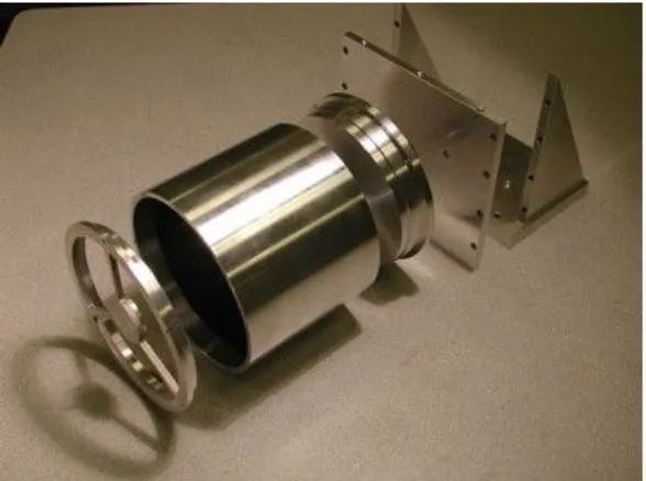
Figure 2-1: Rough machined components of the two-mirror telescope.

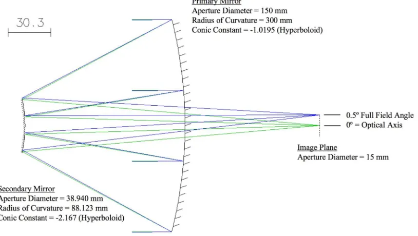
Figure 2-2 shows the optical path of the final telescope design and gives the

specifications for the hyperbolic mirrors as described by Wanna [25]. The design

requirements for the Ritchey-Chrétien called for a primary with f/number = f/1 for high

light-gathering ability (f/number = aperture diameter/focal length), a 150 mm primary

mirror aperture, a 15 mm detector height, 1º total field angle (± 0.5º) and 20% secondary

mirror obscuration (distance from the primary focal point as percentage of primary focal

length). For a concave mirror reflecting a collimated wavefront (infinite conjugate) the

radius of curvature is twice the focal length; so for a f/1 primary with 150 mm aperture

(27)

Figure 2-2: The optical path of the Richey-Chrétien telescope with optical elements and

specifications. Incident light from the object (infinite conjugates) enters from the left and

the image is formed on the right. Path generated with OSLO-EDU® from Lambda

Research Corporation.

To create the optical surfaces, the tool moves through the prescribed hyperbolic path

(from the outer radius to spindle centerline) with some compensation based on the

circular edge shape of a diamond tool. The geometry (straightness and squareness) and

control system of the machine slides determine the optical shape form error. The circular

tool radius, tool edge quality, speed at which the tool is fed across the part, machine

vibration and workpiece material determine the surface finish.

(28)

Fiducial surfaces are used to locate the two mirrors with respect to each other as

prescribed by the optical design specifications. In this two-mirror system, a step on OD

of the primary mirror locates one end of the tube while a step on the OD of the secondary

support structure locates the other. The distances between the optical apexes and fiducial

steps, combined with the length of the tube, set the mirror spacing. High resolution (2.5

nm) length measuring laser interferometers mounted on the DTM slides were used to

control these distances during machining. Figure 2-3 shows a cross section of the

components with heavy lines to indicate surfaces that were diamond turned. The

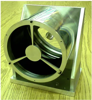
assembled system can be seen in Figure 2-4.

Figure 2-3: Cross section of telescope components with dark lines indicating surfaces

(29)

Figure 2-4: Final assembled optical system.

2.2 M

ATERIAL

P

REPARATION

2.2.1 Rough Machining

The telescope components shown in Figure 2-1 were rough machined with allowances for

diamond turning of the optical and fiducial surfaces. The drawings of the rough

machined components are found in Appendix C. All surfaces diamond turned had at

least 150 µm of extra material that was removed during final machining. The optical

(30)

primary and secondary mirrors each have a tapered OD to align their centerline with the

tube centerline when assembled. Rough machining of the step was specified at 90º so it

had the extra 150 µm plus the material removed to create the taper. The interior of the

tube was anodized black with a matte finish to minimize internal reflections.

2.2.2 Heat Treatment

To relieve residual stresses introduced during the rough machining process, the

components were heat-treated. The procedure was as follows:

1. Cool the parts in a -100 ºF environment at a natural rate for one hour.

2. Warm to room temperature in a still, ambient atmosphere.

3. Heat in a 300 ºF environment at a natural rate for 2 hours.

4. Cool to room temperature in a still, ambient atmosphere.

5. Repeated steps 1-4 once.

2.2.3 Material Hardness

(31)

!

VHN=1.72P

d2 (2-1)

All tests were performed using a 1 Kg load, which is well suited to the hardness of

machined aluminum because it provided small indention marks (0.1 mm) that had crisp

edges and corners. Increasing the load would cause a larger indention and the original

surface would extrude upward at the indention edge.

Three pieces were tested: the heat-treated spacer and two reference specimens of

6061-T6. The diagonal lengths of the indention were measured with two methods on the Zygo

NewView white light interferometer and its software, MetroPro. The first method

measured the diagonal lengths on an interferometric image with manually drawn trace

lines across the indenture corners. MetroPro reported the trace length. The second

method utilized the translating stage to align a cross-hair on the video monitor with each

corner. MetroPro reported the X and Y position of the stage (crosshair) when aligned

with a corner and the diagonal lengths were calculated using the Pythagorean theorem.

This yielded two diagonal lengths for each method and the average of all four

measurements was used to calculate the VHN. The resultant indentation lengths and

(32)

Table 2-1: Vickers Hardness Values for Rough Machined Telescope Components

Sample Diagonal (mm) Hardness (VHN)

Equation 2-1 (kg/mm2) Hardness (GPa)

Spacer 0.125 110 0.110

Reference 1 0.139 90 0.90

Reference 2 0.126 108 0.108

The published hardness of 6061-T6 Aluminum is 107 VHN or 95 Brinell hardness [18].

Both the spacer and Reference 2 are close to this value but Reference 1 is lower. None of

the samples approach the hardness of un-tempered 6061: 30 Brinell hardness. Based on

the results shown in Table 2-1, the heat treat process used to relieve residual stresses from

rough machining had no effect on the hardness of the optical surfaces.

2.3 DTM S

ETUP

2.3.1 DTM Geometry

The fabrication of axisymmetric, Richey-Chrétien optical systems can be carried out

using a t-based Diamond Turning Machine (DTM) shown in Figure 2-5. It is a

(33)

of the primary mirror for vacuum chucking. The diamond cut back of the primary is then

vacuumed to the spindle and the fiducial surface is machined during the same setup that

cuts the optical surface. The distance between the fiducial surface and the apex of each

optical surface is set during the single part chucking. After the primary is removed, the

secondary is mounted and machined in the same manner with the same tool setup. The

tube is then machined with a different tool layout because of is length and inner diameter

fiducials. The tube length, face parallelism, and ID alignment set the relative position of

the two optical elements. While the tube shown in Figure 2-6 is only one way to create

the spacing between elements, it is a good illustration of the technique used to build

rotationally symmetric systems because lengths and diameters are controlled with the

(34)

(35)

Figure 2-6: Fabrication of Richey-Chrétien telescope components on the ASG-2500 DTM

with a dashed line to show the collinear optical, tube and spindle axes.

2.3.2 Tooling Setup

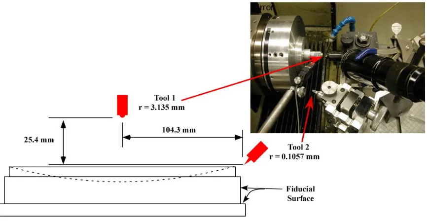
To create both the optical surface and the fiducials in one setup, two tools were used: a

large nose radius (3.135 mm) for low optical surface roughness with shorter machining

times and a small radius tool (0.1057 mm) for the sharp corners at the intersection of the

fiducial surfaces on the primary and secondary. The DTM X-axis table provides room for

multiple tool holders. Figure 2-7 shows the orientation and relative distance between the

tools that was necessary to insure that neither contacted the workpiece while the other

was in use. The tool holders and diamond tools were situated in this fashion before they

were aligned to the DTM coordinate system. The small radius tool is angled towards the

spindle centerline (angle set at ~ 30º for adequate tool holder clearance) as seen in Figure

2-6 so that it can machine both the fiducial OD and step. The complete fiducial

machining path is discussed later in Section 2.5.3 through 2.5.5. Since the back of the

primary mirror is mounted to the spacer plate, overall thickness is a critical feature. It was

then necessary to simultaneously know the position of the both tools with respect to the

(36)

Figure 2-7: Tool layout on the DTM illustrating the relative location of the two tools and

the 10x telescope (black cylinder on right of photo).

The X and Y position of each tool apex were located relative to the spindle centerline

while the Z positions were located relative to the vacuum chuck face. Both tools were

aligned to the spindle axis in the Y and X directions within 1.5 !m. The absolute

positions of each tool in the X direction were recorded so that they could easily be

switched between during machining.

(37)

in Section 2.3.2 shows the larger tool being centered with respect to the spindle

centerline. For fine centering errors in the horizontal direction (short or long in the X

direction) an “Ogive Error” appears in the surface profile as measured with the laser

interferometer [2]. Ogive error is named so because its characteristic shape often appears

in arches of Gothic architecture and is seen in Figure 2-8. Gerchman discusses centering

errors and calculated that the impact on form error is much greater for horizontal errors

(X-direction) than vertical errors (Y=direction) [2]. It has been shown by others that the

horizontal centering error can be modeled by adding an offset to the radial position in the

standard aspheric sag formula [34].

Figure 2-8: Ogive error caused by tool going past spindle center in X direction.

The technique used here was a multi-step method where several cuts in a centering plug

(38)

step (first cutting stage) set the rough center by finding the center error in both directions

simultaneously because large errors are difficult to separate into X and Y components.

The third stage of alignment sets the final tool center through error shapes seen in the

centering plug and features seen at the tip. This stage generally requires several iterations

and with each iteration, the X and Y direction errors are reduced independently of one

another.

2.3.3.1 Step 1: Visual Alignment at Setup

A centering plug in its holder is seen in Figure 2-9. An obvious feature may still be

visible at the center of the plug through the 10X telescope if a previous centering exercise

had a large height error (Y direction). If the small feature is visible (with the spindle

running), the initial centering in the X direction can be accomplished by aligning the tool

apex with the feature while looking through the telescope. If no feature was visible,

initial X center was set by simply judging the apex of the tool with respect to the Z-axis

(best done while standing behind the tool and looking towards the chuck face) and

aligning it with the center of rotation. Both of these techniques yield alignment between

spindle centerline in the X direction and the tool to within 500 !m.

(39)

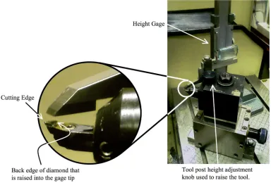
Figure 2-9: Centering plug mounted in holder, which is vacuumed to chuck.

To set the initial tool height (Y direction), a height gage was set to the nominal spindle

height (6.007 in) and tool post was raised until the back edge of the diamond was seen to

touch the gage tip; extreme care must be used here, as it is especially easy to damage the

(40)

Figure 2-10: Height gage used to set the diamond tool height (Y-direction) at setup.

The diamond is raised into gage tip by turning the knob on the tool post.

2.3.3.2 Step 2: Rough Center

Rough centering was accomplished through use of the two-circles method. At larger

alignment errors, the error in the horizontal (X-direction) and vertical (Y-direction) are

not easily separated. Once initial alignment had been visually set, the tool was jogged

(41)

than 2 !m so a few open-loop jog pulses at the slow speed, once the tool has contacted

the part, are adequate. The tool is then jogged away from the part and moved in the

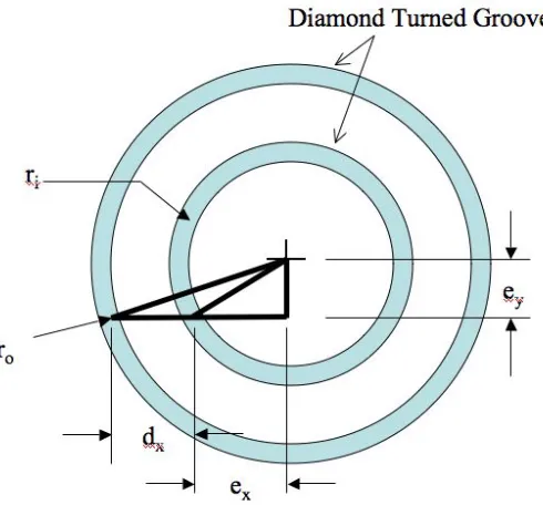
X-direction some distance to create the second outer groove at radius ro. The X-distance

moved is recorded and seen in the Figure 2-11 as dx. The part is removed from the DTM

and the groove diameter is measured with the NewView using the crosshair and

translating stage technique discussed in Section 2.2.3.

Figure 2-11: Two diamond turned grooves cut in the end of a centering plug.

Since the radii of the grooves (ri and ro) and the distance moved in the X-direction (dx)

are known, two equations with two unknowns can be written using the Pythagorean

(42)

with respective hypotenuses of ri and ro that share the common height, ey. Solving for the

two error terms yields the following system of equations:

!

e_x = ro

2

"d_x2"2d_x

2d_x

e_y = r_i2"e_x2

(2-2)

which gave the errors from the current tool location. The new offsets were programmed

into the DTM and the fine centering steps were started.

2.3.3.3 Step 3: Fine Tool Center in the Vertical (Y) Direction

To set the fine position of the tool a small convex sphere was machined on a test part and

measured to find its error shape. This technique requires a few iterations to set the tool

center within 2 !m of the spindle centerline. For centering errors in the vertical direction

(low or high in the Y direction), a center defect will be created and the micro-height

adjustor can be used to center the tool in the Y direction. The center defect was measured

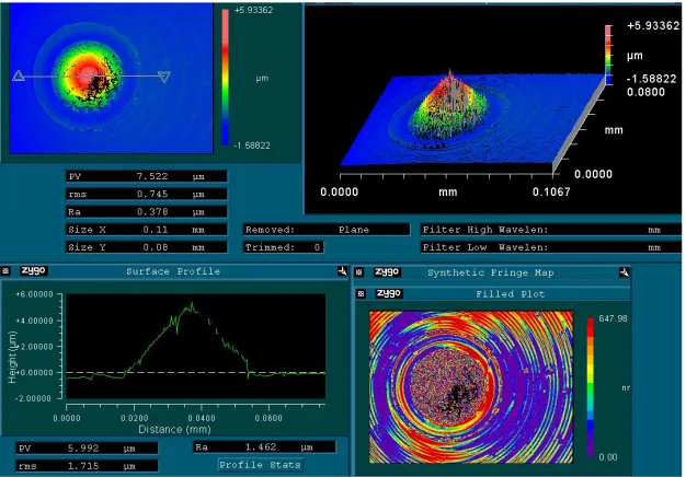
with the Zygo NewView white light interferometer. If the tool is lower than the spindle

centerline, it simply fails to remove a small portion of material that is shaped like a

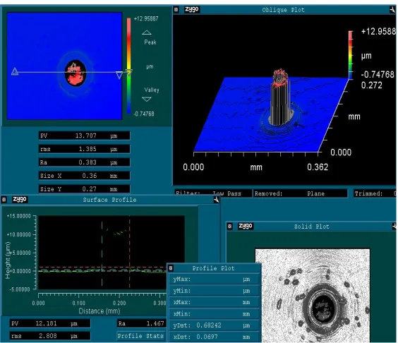
cylinder as seen in Figure 2-12. If the tool is higher than the spindle centerline, a defect

(43)

Figure 2-12: Screen capture of the New View measurement showing a centering error in

(44)

Figure 2-13: Screen capture of the New View measurement showing a centering error in

the vertical direction (Y). The cone shape indicates the tool was high of centerline.

When working with small center features or center features without a clear shape, marks

left on the workpiece from seams in the spindle air-bearing pads are useful to determine

the direction and magnitude of the vertical error. When the spindle shaft passes a seam in

air-bearing pad, it moves the chuck and workpiece into the diamond tool. This spindle

motion is synchronous and is sometimes called ‘spindle star.’ Figure 2-14 shows the

spindle star and has lines overdrawn to show the relationship between two marks that are

180º apart (there are 12 pads which make 12 marks so there are 6 opposing pairs). With

(45)

Figure 2-14: Spiral at center of workpiece where radial lines created by spindle

air-bearing pads are visible. Dark lines highlight two opposing marks that, with counter

clockwise spindle rotation, indicate tool was low.

2.3.3.4 Step 3: Fine Tool Centering in the Horizontal (X) Direction

Figure 2-15 shows the form error for X-direction errors where the plug shapes are at the

top (dashed line indicates tool path) and the error shapes with respect to a best-fit sphere

(46)

value of X corresponding to the aperture radius to the programmed point of X=0 and the

tool goes beyond the spindle centerline, the interferogram will have the Ogive shape as

seen in Figure 2-15a. If it stops short of the spindle centerline the interferogram will

have a wavy dip in the center as seen in Figure 2-15b. The peak in the center of the error

in Figure 2-15b is caused by the center feature remaining when the tool stops short and, if

the error is small, is not always observed in the part measurement. For a concave sphere

test part, the ogive error shapes are inverted about the best fit sphere line.

a) Long of Center in X-direction b) Short of Center in X-direction

Figure 2-15: Cross Sectional Error Shapes for a Centering Plug Sphere in the Horizontal

Direction (X).

(47)

the spindle centerline is seen in Figure 2-16 and the error shape can be matched to the

one seen in Figure 2-15a.

Figure 2-16: Screen shot of GPI output showing a centering error in the horizontal

direction (X) where the tool was long of center. Trace shape seen in Figure 2-15a.

2.3.4 Tool Z reference

After the tools were centered with respect to the spindle axis (X and Y), each apex was

referenced to the face of the vacuum chuck to define a common Z reference. By setting

(48)

X=Y=Z=0, the Z direction offset could be easily found by bringing the tool into contact

with the vacuum chuck. The small tool was used to face the vacuum chuck to ensure that

no raised material that would influence mirror fabrication. The large tool was “touched”

to the chuck using a closed loop program with 100 nm step sizes. Because the tool radius

was large, even a depth of cut of 100 nm produced a chip large enough to see with the

10x telescope seen in the bottom right of the photo in Figure 2-7. The Z-axis offsets of

each tool were recorded after they were referenced to the spindle face so they could be

switched between while performing various operations on the ASG-2500. As discussed

later in Section 2.5.1, the chuck had a convex shape with a peak to valley error of about

700 nm due to squareness error between the slide axes. The large tool was touched to the

chuck at an intermediate radius, so the error in offsets was about 350 nm.

2.3.5 Surface Finish, Feed Rate and Spindle Speed

Feed rate and spindle speed are selected based on the desired surface finish, machining

time and error characteristics of the spindle. The theoretical peak-to-valley (PV) surface

finish is calculated from Equation 2-2 with a parabolic approximation of the tool shape

(49)

!

PV = f 2

8R_t (2-2)

Smaller feed rates and larger tool radii will improve the finish. However, there is a

roughness minimum that is based on the asynchronous vibration of the spindle, the tool

sharpness and the material to be machined. Asynchronous spindle vibration will change

the cutting depth from one revolution to the next for any angular position across the face

of the part thus increasing the surface roughness. The tool edge sharpness will affect the

minimum chip thickness and can increase the roughness [12, 13]. Finally, the material

structure (for example second phase particles in 6061 Al [10, 11]) will create

imperfections that will degrade the surface finish. The sharpness of the tool can interact

with the second phase particles in 6061-T6 and a less sharp tool can produce better

surface finish than a sharp one [12].

For the proposed mirror surfaces, a spindle speed of 530 rpm was selected (minimum

error motion as measured), feed rate of 2 mm/min for the primary, 1 mm/min for the

secondary, and a tool nose radius of 3.135 mm. At these feed rates, each finish pass was

approximately 40 minutes long, indicating the need for excellent temperature control

because of the temperature sensitive of the laser interferometers in the ASG-2500 [5].

For these machining conditions the theoretical PV surface roughness from Equation 2-2

will be 0.57 nm for the primary and 0.19 nm for the secondary. The ASG-2500 has

created surface finishes on the order of 2 nm in pure materials (plated copper and 1100

(50)

RMS due to the issues discussed above which are further explored in the Chapter 4 of this

thesis.

2.4 C

ONTROLLER

P

ROGRAMMING

2.4.1 Number of Points in the Programmed Path

The hyperboloid surfaces of the primary and secondary mirrors are created with a

programmed path that consists of a series of X, Z commands. As a result, the controller

prescribes a series of straight lines that approximate the hyperbolic shape. If the

acceptable deviation between the programmed straight lines and curved tool path is 1 nm

and the reflective surface is approximated as a parabola, Equation 2-2 can be used to

calculate the acceptable distance between points for the primary mirror. Equation 2-3

shows Equation 2-2 solved for f, where f = dp is the distance between points along the

straight line, PV is the peak-to-valley sag between the line and curve it represents, and Rt

is the parabolic base radius. The cutting path length of the primary mirror is 62 mm, so

62 mm divided by 48.9 !m/point yields 1266 X, Z points. Employing the same method

for the secondary mirror yields 735 X, Z points.

(51)

2.4.2 Tool Radius Compensation

The shape of the diamond tool must be considered when cutting non-flat surfaces. For a

circular tool cross-section, the theoretical tool center traces out a path that is offset from

the cutting edge by the radius of the tool as seen in Figure 2-17. The direction of this

offset is perpendicular to the slope of the surface at the point of contact. The tool radius

was measured using the translating stage and video output of the NewView to position a

crosshair on the diamond edge. The MetroPro software gives coordinates of the stage

(taken as the coordinates of the crosshair) and, with several points recorded along the

cutting window, the data are input to a curve fitting function in MATLAB to find the best

fit radius.

Figure 2-17: Illustration of surface normal vectors and tool offset to form discrete tool

path. Desired surface is a continuous function and the normal vector length is equal to

(52)

The programmed tool path can be corrected for the radius of the tool by finding the

normal vector at each point in the path and offsetting the axes locations by the tool radius

along this vector (in the correct direction). Figure 2-17 shows a hypothetical surface

shape with evenly spaced normal vectors that are equal in length to the radius of the

diamond tool in that figure. The dashed line represents the discrete tool command, which

is a series of straight lines between successive points as discussed in the previous section.

The discrete tool path length between the two right most normals is smaller than the

length between the left most normals because the curvature between the right most

normals is greater. Normal vectors can be found analytically for geometrical surfaces or

estimated numerically for a closely spaced path of discrete data points. The offset for

each discrete point is simply the product of the tool radius with the sine (for X) and the

cosine (for Z) of the normal angle. Figure 2-18 shows the desired primary surface (solid

line), the tool radius compensated machining path (dashed line), and has three circles

(53)

Figure 2-18: Cross-section of desired primary optical surface (solid line) and tool radius

compensated machining path (dashed line) with circles representing the tool radius. To

scale.

The sequence of corrected points defines the commanded path of the tool center. The

result of this process is illustrated in Figure 2-19 where the upper curve in each plot

labeled “Tool Path” (i.e., the tool center) is at a constant offset (the tool radius) from the

hyperbolic surface swept out by the tool edge during machining. The upper curves are

the recorded tool paths as measured by the laser interferometer and are discussed in the

next section. The same data uncompensated for tool radius is shown as dots and the

(54)

Figure 2-19: Primary (upper) and secondary (lower) mirror motion plots drawn by K.

Garrard. The circles (o) identify the uncompensated tool pathwhile lines passing through

the circles labeled Hyperbola are the surface as specified by the optical design. Lines

labeled Tool Path are the tool radius compensated path.

2.4.3 Axes Following Error

(55)

every 32nd iteration of its 500 Hz servo loop, for a 15.625 Hz sample rate (64 milliseconds/sample). The finish pass cross-feed rates for the secondary and primary

mirrors were 1 and 2 mm/min, respectively. Approximately 30,000 data points were

collected for the primary mirror motion program and 22,000 data points for the secondary

mirror. Each sample contains the commanded positions of the X and Z axes, their actual

positions as measured by the laser interferometer, and the servo loop voltage commands

sent to the pulse width modulated motor amplifiers. This is the data seen in Figure 2-19

and Figure 2-20. Each axis of the DTM vibrates at its natural frequency (Z axis with

spindle is 64 Hz and X axis is 89 Hz) with amplitude of about 30 nm [12, 13, 14] but this

vibration will appear as aliased high frequency information in the sampled data because

the Nyquist frequency of the sampled data is 7.8126 Hz [29]. In Figure 2-20 this aliased

high frequency vibration was removed with a 100 point running average filter.

The error in tool trajectory caused by the control system for each mirror is a combination

of the X and Z command following errors. To evaluate this error, X and Z axis positions

were compared with the ideal trajectory in Figure 2-19. As discussed previously, the

commanded tool path and the resulting motion of the axes were compensated for tool

radius. The direction of the offset is determined by whether the shape is a concave or

convex. Therefore, to compare the actual motion to the desired path, the recorded data

was uncompensated for tool radius by applying a radius compensation algorithm in a

direction normal to the tool path and toward the ideal surface. Then, for each X position

in the data set, a sag value on the desired hyperbola was generated and the sag error was

(56)

Figure 2-20 shows the difference between the dots and the solid lines that pass through

them from the two plots in Figure 2-19. This difference is the sag error as recorded by

the ASG-2500 control system laser interferometer feedback. For the primary mirror the

PV motion path error is 16.75 nm (2.4 nm RMS) and for the secondary mirror the error is

12 nm PV (2 nm RMS). The pitch of the lead screws is 5 mm and neither plot exhibits

that spatial frequency because the laser interferometers measure in the direction of axis

motion as discussed later in Section 3.2.2. At the relatively slow feed rate used to

machine both mirrors, the dead band from the controller DACs, ball screw friction, and

motor friction were most likely responsible for the error magnitude [32]. The actual tool

motion is close enough to the programmed tool path to create no figure errors.

(57)

2.5 D

IAMOND

T

URNING

O

PERATIONS

The diamond turning machine used for machining the optical and fiducial surfaces is a

Rank-Pneumo ASG-2500 T-lathe and is seen in Figure 2-5. It is equipped with

hydrostatic oil bearing slide-ways, laser interferometer position feedback for slide-way

position (2.5 nm resolution), ball screw slide drives, air bearing spindle with angular

encoder (20,000 points/rev) and a vacuum chuck to hold parts to the spindle. A

controller developed at the PEC is used to command the position of the axes. It uses a

Motorola 68020 processor board with Burr-Brown input/output boards for motion

control. The host PC for the 68020 was an early 1990’s PC-AT 80286.

The fabrication capability of a modern DTM allows the optical elements to be machined

with a form tolerance of !/4 (150 nm) on the optical and fiducial surfaces while

diameters and lengths can be fabricated to a tolerance of ±2 !m. For the R-C telescope

discussed in Section 2.1, machining errors of this magnitude double the wave front error

(0.15 ! to 0.30 !) of the best performing field angle (0.35º) and increase the other field

angle (0º and 0.5º) errors by about 10% (0.7 ! to 0.8 !) [28].

The remainder of this section describes the steps in the fabrication of the mirror and

(58)

2.5.1 Step 1: Vacuum Chuck

2.5.1.1 Flatness

The face of the vacuum chuck was used in the machining process as the reference surface

for position of the optical and fiducial surfaces. It was faced off prior to machining and

was assumed to be flat. Unfortunately, this was not true. Figure 2-21 shows the flatness

of the chuck around the periphery measured with an electronic LVDT indicator by the

PEC staff after the optic was fabricated. Comparing the slope of the flat and tapered

faces, the relative angle is about 2 arc-seconds. This is a result of the spindle axis

(mounted to but not necessarily perfectly aligned with the Z-Axis) to X-Axis squareness

error and not activating the yaw and squareness correction built into the machine tool

controller as discussed in the next chapter. The surface of the chuck was cone shaped

with a peak in the center and the taper had a magnitude of about 710 nm. This lack of

flatness had an effect of the shape of the finished mirrors and suggestions for future

(59)

Figure 2-21: Vacuum chuck flatness (left) and runout (right) as measured for two mirror

fabrication.

2.5.1.2 Axial Runout

The axial runout of the chuck was also measured with a LVDT indicator while the

spindle rotated at low speed and is shown at the right in Figure 2-21. The indicator was

80 mm from the center of the spindle (spindle radius is 101.6 mm). The peak-to-valley

runout is low (140 nm), which should produce an optical surface that has less than #/4

non-rotationally symmetric error. If this value is deemed too high, the chuck could be

machined with the FTS or a workpiece aspect ratio could be designed to tolerate this

(60)

2.5.2 Step 2: Primary Back

The back of the rough machined primary mirror was diamond turned to create a flat

reference surface for attaching it to the vacuum chuck. The back of the primary is seen in

Figure 2-22. A small flat ring was first cut into the outer rim of the optical surface (front)

to create a chucking surface. When this component was vacuumed to the chuck, the

support at the edge would cause it to take on a concave shape. If machined flat and

removed from the chuck, it would elastically deflect into a convex shape because the

aspect ratio was low of (thickness to diameter = 1:6) [28]. However, the tool path could

be modified to counteract this effect. The shape of the back while the primary vacuumed

to the chuck was measured (~0.7 !m concave) with an LVDT indicator with involute tip.

The back was measured off the chuck (1.3 !m convex) and then machined with a

concave radius that had sag equal to 2 !m. When the back was inspected after the first

pass, an edge of the surface remained uncut which indicated the rough machined

component was non-rotationally symmetric, so the operation was performed again with a

larger depth of cut. The final shape of the primary found in Woodside’s measurements

[1] shows a convex shape with about 0.6 µm of magnitude. The convex shape in the

vacuum chuck described previously in Section 2.5.1 would indicate that the machine axes

were not square for this operation and explain why the back of the primary had a convex

(61)

workpiece contained non-rotationally symmetric distortion. Future suggestions to

address this issues are discussed in Section 2.5.7.

Figure 2-22: Diamond turned primary back. Center plug is rubber.

2.5.3 Step 3: Primary Mirror and Fiducial

The programmed path of X, Z commands is based on the mathematical description of the

optical surface. The optical surface is a hyperbola with a k=-1.0195, a base radius of 300

mm, an OD of 150 mm and a 26 mm hole in the center. Because there is a hole in the

(62)

optical surface was first rough machined to the desired hyperbola shape with the 0.1057

mm tool (used for the fiducials, not the optical surfaces) to preserve the edge sharpness of

the 3.135 mm tool. When cutting 6061-T6 aluminum, second phase particulates cause

high tool wear rates and can easily damage a sharp nose radius [8,12,13]. The finished

optical surface was cut using the 3.135 mm tool and multiple passes were performed at

increasing depth until the surface was completely machined. At this point, machining

logs indicated that apex to chuck distance was 22.571 mm. The designed distance was

22.5 mm; however, tool wear concerns dictated the decision to cease machining at the

larger thickness. Fiducial step height was adjusted accordingly so the relationship of the

fiducial step to the apex was preserved at 15 mm and there was no impact on the distance

from the primary apex to the secondary apex (measurements indicated that machining

error between the fiducial and apex were 3 !m [33]). Because the overall thickness of

the primary was larger, the relationship between the system apex and the

camera-mounting surface was affected. Adjusting the spacer washers between the primary and

the spacer plate could compensate for this difference.

The cutting paths are seen in Figure 2-23. Unfortunately, the tool radius was input to the

controller as 3.125 mm instead of the measured radius of 3.135. As a result, sag in the

(63)

Figure 2-23: Primary optical and fiducial cutting paths.

The fiducial feature that transfers the primary optical shape to the secondary is a step on

the OD that mates with the tube and is shown in Figure 2-23. Figure 2-24 shows the

critical features of this fiducial: the taper angle (1º), the taper radius and the step height

from the vacuum chuck. This feature was machined with the 0.1057 mm radius diamond

tool, which was set to Z reference and spindle centerline as discussed in Section 2.3.3 –

(64)

Figure 2-24: Cross-section of Primary showing critical fiducial features. Surfaces cut

are drawn with bold lines.

Cutting parameters used for the primary were dependant on machining operation. For

machining the optical surface with the fiducial tool, a feed rate of 25 mm/min and a cut

depth of 25 !m was used to reduce the time needed for each pass. 7 passes were required

to create the hyperbolic shape. For rough machining of the fiducial, the feed rate was 10

mm/min and cutting depth was 20 !m. The final pass on the fiducial was done at 1

mm/min. The final depth of cut for both surfaces was 1 !m and the spindle speed was

(65)

extend to a ring that mates with the tube via the same interference fit method as the

primary. As with the primary, to guarantee axisymmetric features the optical surface and

the fiducial were diamond turned sequentially without removal from the vacuum chuck

between operations. The diamond turned secondary is seen in Figure 2-25.

Figure 2-25: Secondary mirror and support structure after diamond turning.

To vacuum this mirror to the spindle, a thin plate with a hole in the center (to allow the

optical surface to protrude) was used to seal the area between the outside ring and the

(66)

ring and a ridge on outside the mirror surface; all three were co-planer and the ridges are

shown in Figure 2-26.

Figure 2-26: Secondary on Vacuum Chuck with Vacuum Plate. Critical Fiducial

Surfaces are in Bold.

The machining processes for the critical surfaces were performed in the same manner as

those used to fabricate the primary mirror because the secondary was designed with

almost identical fiducials. The critical features were the step height from the chuck to

Surface Finish and Form Fidelity in Diamond Turning

ABSTRACT

Surface Finish and Form Fidelity in Diamond Turning

by

Donald Lucas Lamonds

DEDICATION

BIOGRAPHY

ACKNOWLEDGMENTS

TABLE OF CONTENTS

LIST OF FIGURES

LIST OF TABLES

1 INTRODUCTION

1.1 B

1.2 P

R

1.3 P

R

PEC

1.4 P

S

2 FABRICATION OF TWO MIRROR TELESCOPE

2.1 I

2.2 M

P

2.3 DTM S

2.4 C

P

2.5 D

T

O