doi:10.1209/0295-5075/94/54005
Sound propagation and force chains in granular materials
E. T. Owensand K. E. Daniels(a)
Department of Physics, NC State University - Raleigh, NC 27695, USA
received 15 December 2010; accepted in final form 26 April 2011 published online 27 May 2011
PACS 43.25.+y– Nonlinear acoustics PACS 45.70.-n– Granular systems
PACS 46.40.Cd– Mechanical wave propagation (including diffraction, scattering, and dispersion) Abstract– Granular materials are inherently heterogeneous, leading to challenges in formulating accurate models of sound propagation. In order to quantify acoustic responses in space and time, we perform experiments in a photoelastic granular material in which the internal stress pattern (in the form of force chains) is visible. We utilize two complementary methods, high-speed imaging and piezoelectric transduction, to provide particle-scale measurements of both the amplitude and speed of an acoustic wave in the near-field regime. We observe that the wave amplitude is on average largest within particles experiencing the largest forces, particularly in those chains radiating away from the source, with the force-dependence of this amplitude in qualitative agreement with a simple Hertzian-like model of particle contact area. In addition, we are able to directly observe rare transiently strong force chains formed by the opening and closing of contacts during propagation. The speed of the leading edge of the pulse is in agreement with the speed of a one-dimensional chain, while the slower speed of the peak response suggests that it contains waves which have travelled over multiple paths even within just this near-field region. These effects highlight the importance of particle-scale behaviors in determining the acoustical properties of granular materials.
Copyright cEPLA, 2011
Introduction. – Sound propagation in granular mate-rials differs from propagation in ordinary elastic matemate-rials in that there is a poor separation of length scales, particu-larly manifest in the branching networks of force chains which transmit stresses between particles. Continuum models [1–3], including effective medium theory (EMT), have failed to quantitatively describe important features. One such deviation from EMT is manifest in the low pressure scaling of the sound speed, which increases with pressure faster than expected [4–6]. Particle-scale changes in the coordination number and force chains are likely responsible for important deviations from these models, and have been the focus of numerical simulations on model amorphous systems near jamming, where soft modes are important [7–9].
Hertzian contact theory underlies models of sound propagation, whether as the interaction potential between particles in discrete element simulations [10] or in the calculation of an effective bulk modulus in EMT [1]. The contact force f between two particles is given by an equation of the formf∝δβ, whereδ is the distance each
(a)E-mail:kdaniel@ncsu.edu
particle is compressed and the exponent β depends on the particle geometry. Two common idealized situations are β= 3/2 for spheres and β= 1 for cylinders. The contact area a between the particles, which in EMT are permanently bonded, has a force dependence given by
a∝f1β, for a circular contact area in the case of spheres, anda∝f21β for a rectangular contact area in the case of cylinders. The sound velocitycis governed by the stiffness
s= df /dδof the contacts; for Hertzian contacts, this iss∝ δβ−1∝fβ−β1. In experiments on one-dimensional chains of identical spheres, [11] observed quantitative agreement with the expectedc∝√sfor a variety of materials.
(d) t = 3.1 ms (c) t = 1.9 ms
driver
(b) t = 0.6 ms
(a)
Fig. 1: (a) Image of photoelastic granular aggregate viewed through circular polarizers. (b)–(d) Representative|∆I|measured within the region marked by the box in (a). The dark background shows the static-force chain network, with|∆I| overlayed on top. White areas represent the areas with the largest change in intensity. A movie of the dynamics is available, see Owens Daniels EPL2011.mp4.
such particle asperities and contact rearrangements are minimized [2,4,13]. However, nonlinear and non-affine effects prevent EMT from providing a complete treatment of the dynamics [6].
An additional complication lies in the observation that
c can take different values within the same system, depending on whether the speed measurement is taken for time-of-flight, peak response, or harmonic excitation [14]. From this property of c, as well as the observation that a minute expansion of a single particle can cause large shifts in the acoustic response, [14–16] proposed that the underlying force chain network is at the heart of the failures of EMT. Simulations by [17] directly addressed the heterogeneity and local dynamics using discrete element simulations of soft spheres. In simulations of a system of idealized Hertzian spheres (β= 3/2), the propagating wave was coherent and insensitive to the force chain network. Reconciling the failures of EMT with this unexpected insensitivity to the force chain network requires measurements of the propagation dynamics in real systems at length scales comparable to the particles and force chains.
In order to address the particular role played by the inter-particle contacts and forces, we make spatiotempo-rally resolved measurements in an experimental system in which changes in the force chain network are rendered visible. Our apparatus is filled with a two-dimensional (2D) aggregate of photoelastic [18,19] disks, allowing direct visualization of the sound path via polarizing filters and a high-speed camera. In addition, piezoelectric sensors embedded in a subset of the particles provide the higher temporal resolution necessary for speed measurements. This combination of techniques allows us to directly measure force, sound amplitude, and sound speed on the particle scale. We observe that the force chain network plays a key role in sound propagation, with the largest amplitude sound propagating along the strongest force chains. We find that a simple model of increasing contact area with inter-particle force provides quantitative agree-ment with the observed trend. In addition, we find while
the sound speed of the leading edge of the signal in our 2D system is consistent with the speed found along a 1D chain, the speed of the peak response is significantly slower. We use this result to explain the speed difference previously observed in 2D and 3D systems [14] by postu-lating that the leading edge of the signal travels only along the stiffest (fastest) path, while the peak response is a combination of sound that traveled along multiple paths and would therefore be independent of the force and slower than the leading edge of the signal.
Experiment. – Our apparatus consists of a (29× 45) cm2 vertical aggregate of O(103) photoelastic disks confined in a single layer between two sheets of Plexiglass (see fig. 1(a)). A pair of left and right circularly polarizing filters on opposites sides form a polariscope, so that particles with larger force appear brighter and with more fringes. The particles are cut from Vishay PhotoStress material PSM-4, with diameters d1= 9 mm and d2= 11 mm in equal concentrations ( ¯d≡10 mm); the zero-frequency Young’s modulus of the material isE0= 4 MPa and the density is ρ= 1.06 g/cm3. Because the particles are viscoelastic, they have a stress-dependent dynamic modulus E(ω); for the 750 Hz signals used here, E≈50 to 100 MPa (see footnote 1). The upper surface of the aggregate is free and we perform measurements near the bottom, where the Janssen effect [20,21] eliminates vertical gradients in the average pressure. The measured pressure at the center of particles ranges from 1 to 20 kPa (small compared to E) and the system has an average packing fraction of φ= 0.84±0.01. To improve statistics, we perform experiments in 19 different particle configurations.
0 5 10 15 20 10−5
10−4 10−3 10−2
r (cm) A∆I AV
0 5 10 15 20
0 1 0 1 0 1
time (ms)
piezo V(t)
photoelastic ∆I(t)
driver (a)
∆tr ∆tp (b)
Fig. 2: Sample signals showing correspondence between two measurement techniques. (a) Driver current (bottom), ∆I(t) for a representative photoelastic particle (middle) and piezo-electric voltageV(t) (top), with all values normalized to same scale. Gray bars illustrate the intervals ∆trand ∆tp. (b) Decay
in average signal amplitude with distance from driver:A∆I(r) for the photoelastic signal (
◦
) andAV(r) for the piezoelectricsignal (). Solid lines showA∝exp−r/ξ withξ= 2.3 cm. Inset: particle with embedded piezoelectric sensor.
of 5 consecutive sine waves with a frequency of 750 Hz, which corresponds to a wavelengthλ= 10 ¯dto 20 ¯d(based on the sound speed measurement presented below). The amplitude of the sound waves is approximately 800 Pa at the driver. Prior to each experiment, we send an annealing sequence of 30 pulses so that the system settles into a state for which we observe repeatable measurements.
We observe the wave propagation through the aggregate using two techniques: the photoelastic response via a digital high speed camera, and the electrical response of particle-scale piezoelectric sensors embedded in a subset of particles (see fig. 2(b)). The former provides data at all particle locations, but only 4 kHz temporal resolution; the latter provides data at only 12 particles but 100 kHz temporal resolution. In addition, a 3k×2k digital camera provides higher spatial resolution images for measurement of particle positions and forces.
We image the photoelastic response of the aggregate using a Phantom V5.2 camera operating at 4 kHz with 512×512 resolution. Since the change in the photoelastic signal during the pulse is weak, maximally ±10 out of 256 levels, we transmit the 5-wave pulse 50 times at 20 ms intervals to allow the previous pulse to dissipate. The frame-by-frame average intensityI(x, y;t) of these 50 pulses is used to measure spatially resolved dynamics. In each frame, we determine the locations where compression is present by examining differences in the image brightness with respect to the initial frame, ∆I(x, y;t)≡I(x, y;ti)−
I(x, y;t0), as shown in fig. 1(b)–(d). The fieldA∆I(x, y;t)
records the maximum amplitude observed at each particle location. Note that for a measured speed ofc= 200 m/s, the 4 kHz frame rate averages the photoelastic response over a distance of approximately 5 ¯d in the direction of propagation.
In addition, we utilize embedded piezoelectric sensors to provide higher temporal resolution for a subset of the particles. Piezoelectrics were chosen because they can fit
within a single particle, produce a voltage proportional to the applied stress, and have a frequency response well above the frequencies we measure. Our sensors are 2 mm thick lead zirconate titanate piezoelectric ceramics from Piezo Systems, Inc., cut to 4 mm × 4 mm squares; this adds 30% to each particle’s mass. The configuration of the 12 sensor-particles is shown in fig. 1(a), with the first row 5 cm from the driver and the remaining rows spaced 3.5 cm apart. Since our piezoelectric sensors are only sensitive to stresses applied across their thickness, it is important to orient them so that their face is perpendicular to a line connecting the center of the driver with the center of the sensor. The voltage measured on any particles not in this orientation is corrected with the appropriate cosine factor during post-processing.
During each train of pulses, we record the time-varying voltage produced by each of the twelve piezoelectric sensors (see fig. 2(a)). Due to the high impedance of the piezoelectric sensors, an op-amp buffer and a 10 MΩ resistor are connected in parallel with the piezoelectric to lower the impedance of the circuit and reduce signal crosstalk. Three quantities are measured for each sensor and the driver: amplitudeAV, rise timetr, and the middle
peak timetp. We measure amplitudeAV by fitting a sine
function to the middle three peaks in V(t). We measure
tr as the time at which each signal rises 15% above its
resting value, and tp as the time at which the maximum
value of the middle peak is attained for each signal. The intervals ∆tr and ∆tp are measured for each sensor with
respect to the driver signal, and are used to calculate the speed of soundc along the observed sound path.
The two amplitude measurements, photoelastic
A∆I(x, y;t) and piezoelectric AV(x, y;t) provide
comple-mentary information: the former with better resolution in (x, y) and the latter with better resolution in t. As can be seen in fig. 2(a), ∆I(t) for a single particle shows the expected 5-peaked signal sent by the driver and measured at a nearby sensored particle. In fig. 2(b), for all 19 configurations, we averageAV(r) over the 3 sensors
in each row and azimuthally average A∆I(r). We find
that AV(r) and A∆I(r) empirically exhibit the same
exponential decay, and therefore differ by only a constant of proportionality. This allows us to use the many A∆I
measurements as individual sensors of sound amplitude rather than being limited by the few piezoelectric sensors. Note that this exponential decay is due to the dissipative nature of both the viscoelastic photoelastic polymer and the frictional granular contacts, and suppresses the multiply scattered (coda) response [15,22].
Fig. 3: (a) Detail of force chains approximately 8 ¯d from the driver. (b)|∆I|during sound propagation for the same region. A new contact, marked by the small ellipse, repeatedly opens and closes during each wave cycle while a transiently strong force chain forms to its right.
photoelastic fringes in the vicinity of each contact to provide an empirical estimate of the normal component of the contact force. From these contact forces, we calculate an estimated pressureP at the center of the disk.
Results. –
Contact force law. We directly measure the contact force law for our particles by compressing a single particle between two plates with the force applied along the particle’s diameter. Figure 4(a) shows the measured force for a range of applied displacements. Within a range which corresponds to the typical pressures in the full experimental system, we find that the contact force law is approximately of the form
f∝δ5/4. (1)
While this deviates from the Hertzian prediction that co-planar cylinders follow a linear contact law, we note that slight out-of-plane rotations of the particles lead to imperfect alignment at their contacts. The value β= 5/4 can therefore be interpreted as lying between β= 1 (for rectangular contacts between co-planar cylinders) andβ= 3/2 (for circular contacts between perpendicular cylinders) [23].
Linearity and nonlinearity. The photoelastic parti-cles allow us to directly visualize an important particle-scale nonlinearity present in the system. Due to the non-zero Poisson ratio of the polymer material (ν≈0.5), a particle under dynamic compression expands in the perpendicular direction, potentially creating new (but transient) contacts during the transmission of a wave. The photoelastic particles render the creation of such new mechanical contacts visible, as can be seen in fig. 3. Two particles not in contact in the static image are seen to form a contact in the|∆I|image. The change is associated with the formation of a transiently strong force chain which had been only a weak path in the static image. Both features repeat during each wave cycle, as the contact is repeat-edly opened and closed. This observation that particle contacts can change during sound propagation violates the
10−2 10−1 100
10−1
100
101
δ (mm)
f(N)
5/4
1
0 2 4 6 8 10
0 0.2 0.4 0.6 0.8 1
Ain
<A
V
>
(a) (b)
Fig. 4: (a) Measured contact force law compared with f∝ δ5/4 and f∝δ (solid lines). (b) AV found from all twelve
piezoelectric sensors in a single pack as a function Ain. AV
and Ain are in arbitrary units of pressure, with Ain= 7.8
corresponding to the 800 Pa driving amplitude used for all experiments. Error bars are standard error and the solid line showsAV∝Ain.
well-bonded assumption of effective medium theory [1] because the connectivity of the network transiently changes due to the passage of the wave. Similar, but permanent, changes to the force network were presumably at work in experiments where minute thermal expan-sion [14] or consolidation of loose packs [24] modified the signal coda.
In spite of the inherent nonlinearity of such events, we nonetheless observe an approximately linear response in the average propagation amplitude of the system. As shown in fig. 4(b), we measure the input amplitude Ain
as the pressure generated by the driver as it compresses the particles, and the output amplitude as the average signal AV received by all 12 piezoelectric sensors in a particular configuration. In order to compare AV for sensors at different distances from the driver and subject to different static stresses, we normalize each sensor by its maximum response at the maximum driving amplitude. Since the piston is driven sinusoidally, it has a maximum displacement of δ=Fcoil
ω2m, where Fcoil is the electrical force from the coil (measured via the current), ω is the driving frequency, and m is the mass of the piston plus some effective mass of the system. For a given ω, system configuration, and Fcoil, this unknown mass remains
constant. Therefore,δ∝Fcoilis not only the displacement
of the piston, but also the compression applied to the first particle. Using this relation to provide δ in eq. (1), we find that the applied pressureAin∝Fcoil5/4. As we increase the current to the coil, we can thereby measure AV
as a function of Ain and find an approximately linear
relationship. This suggests that at the driving magnitudes investigated here, the transient contacts are rare events and not a large enough effect to detectably destroy the average linear response.
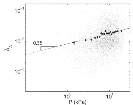
100 101 10−3
10−2 10−1
P (kPa) A ∆
I
~
0.35
Fig. 5: Scatter plot (small points) of amplitude ˜A∆I measured at each particle with positionr <12 cm, as a function of the particle pressure P. The dashed line is ˜A∆I∝P0.35, fit to all points. Large symbols are averages (and standard errors) calculated over several hundred measurements within equally populated bins.
of the wave passing through that particle, where ˜A is corrected for the exponential decay shown in fig. 2(b). As can be seen in fig. 5, particles with higher pressures experience, on average, a larger amplitude. A power-law fit to these points finds ˜A∆I∝P0.35±0.06, where the error in the exponent is reported at a confidence level of 95%. To further illustrate the trend, we sort the measurements by
Pinto 20 equally populated bins and calculate the average A˜∆Iand the standard error for each bin.
We can understand this amplitude trend in terms of the measured contact law in eq. (1). The Hertzian contact area
aformed between two such disks pushed together by a pair of opposing forces f is a∝f2/5. If the contacts between particles are the main conduits for sound propagation, then we would also expect the amplitude of the sound to vary as
˜
A∆I∝P2/5. (2)
This relationship is consistent with the data shown in fig. 5, for which we found an exponent 0.35. However, this contact model is an over-simplification in several important ways. While the Hertzian contact theory was developed for diametric loading, the multiple contacts on each particles arise at various angles. Furthermore, while the sound propagates radially outward from the driver, the force chains form arcs which are not in general aligned with this direction (see fig. 1). As such, a more sophisticated treatment would consider only the radial component of the stress tensor. Finally, as shown in fig. 3, ˜A∆Ican be anomalously large due to the transient changes in the force network. The significant scatter in fig. 5 indicates that eq. (2), while observed on average, is insufficient to account for all effects.
Sound speed. We measure sound speed via the signal travel time from the driver to the piezoelectric sensors
0.2 1 10
50 100 200 300
P(kPa)
c (m/s)
cr cp
5 10 15
P(kPa) r = 5 cm
r = 5 cm r = 8.5 cm
r = 8.5 cm 1/10
(a) (b)
Fig. 6: (Colour on-line) (a) Sound speedscr (◦) andcp() for
a 1D chain of particles. The dashed line is c∝P1/10, which corresponds to the force law given in eq. (1). Error is on the order of the symbol size. (b) 2D sound speeds, cr (•) and
cp(), measured by the piezoelectric sensors as a function of
the average pressure ¯P along the observed path. Large symbols are for sensors atr= 5 cm, small symbols atr= 8.5 cm.
(see fig. 2(a)) along the dominant propagation path from the driver to each sensor from the high-speed movies (see fig. 1(b)–(d)). As in [14,17], we record both the travel time for the initial rise (∆tr) and for the peak response
(∆tp). The distance travelled is taken to be the observed
path (rather than Cartesian distance) since this is the path over which we observed the largest amplitude sound propagates. This path is selected by hand from the movies; we measure the path length L and calculate the two sound speeds, cr=L/∆tr and cp=L/∆tp. In addition,
we measure ¯P as the average P for all particles along the observed path. Due to the exponential decay in the amplitude of the signals, quantitative speed data is only available for the inner two rows of sensors located atrλ. As shown in fig. 6(b),cr andcp are both independent of the distance from the driver, withcrconsistently faster.
To understand the discrepancy between cr and cp, we compare the measured speeds from the 2D system to simpler 1D chains of 11 mm particles confined by a known force within a linear channel centered above the driver. For Hertzian contacts, we expect c∝√s∝fβ2−β1∝f1/10. As shown in fig. 6(a), the measured 1D sound speeds, cr
andcp, illustrate this weak dependence. In the 2D system,
the average value ofcr is in approximate agreement with
the 1D chain values while, the average value ofcpis much
slower than its 1D counterpart. (See Discussion, below, for the significance of this result.)
Additionally, we note that these speeds are faster than the bulk speed predicted by the zero-frequency Young’s modulus (c=E0/ρ= 61 m/s). However, E depends on both the driving frequency and degree of pre-loaded stress due to viscoelastic stiffening. Independent measurements (see footnote 1) of the dynamic E at typical values of ω
andf predict a bulk speedc= 220 to 310 m/s.
Discussion. – The trend of increased sound ampli-tude A along the force chain network is visible qualita-tively in fig. 1 and quantitaqualita-tively in fig. 5. The shape of
contact area (a∝f2/5) under an interpretation in which an increased contact area leads to a larger conduit for sound transmission. Such a trend is in contrast with the lack of amplitude-dependence observed in simulations of idealized (β= 3/2) spheres [17]. This raises the question of whether the discrepancy between experiment and simu-lation might be due to real deformable particles having a behavior different from simulated particles which mathe-matically overlap each other without deforming.
In experiments on sand [14] and in numerical simu-lations [17], the measured value of c depended on the method: the speed at the leading edge of the signal, cr,
was observed to be several times faster than that of the peak response,cp. By definition,cr represents the arrival
of the first signal, that which arrived along the fastest (stiffest) path. This is inherently 1D-like propagation, and measured values of cr for the 2D system are in
approx-imate agreement with 1D measurements. The behavior along each segment of force chain may be reminiscent of sound propagation in 1D granular chains [11], but with a network of connections between the chains. In contrast, the peak response measured bycp is composed of signals which have travelled via many different paths, all of which are by definition longer and/or slower than the fastest path. This may be related to simulations which showcp
saturating to a maximum value as a function ofr[25]. Note that these experiments are performed within a near-field regime (r < λ) on a highly dissipative viscoelas-tic material. The viscoelasviscoelas-ticity only affects the constant of proportionality inf∝δβ, whileβ depends only on the contact geometry. However, it is possible that viscoelastic stiffening enhances the importance of the force chains. In spite of these limitations, the use of these photoelastic materials permits us to address the importance of particle-scale heterogeneities to sound propagation, and the appli-cation of these techniques outside the near-field regime will require the use of less-dissipative materials.
Conclusions. – In conclusion, we observe that the local amplitude of sound waves is influenced by the force chains, and that these chains may in rare cases change due to the transmission of the sound pulse. This highlights the role of force chains as more than just a contact network between grains. Local properties of the material are crucial to local sound propagation dynamics, and mean-field models therefore are unlikely to capture the full behavior of the system. The dependence of these results on the wavelength of the disturbance [26], either above or below the length scale set by the force chains, may provide a means to acoustically probe the force chain network in non-photoelastic 3D systems.
∗ ∗ ∗
The authors would like to thank C. Daraio, P. Johnson, E. Somfai, and N. Vriend for helpful discussions, and C. Chafinand S. Couvreurfor devel-opment work on the project. This work was supported by the National Science Foundation (DMR-0644743).
REFERENCES
[1] Digby P. J.,J. Appl. Mech.,48(1981) 803.
[2] Goddard J. D., Proc. R. Soc. London, Ser. A, 430 (1990) 105.
[3] Velicky B. and Caroli C., Phys. Rev. E, 65 (2002) 021307.
[4] Jia X., Caroli C.andVelicky B.,Phys. Rev. Lett.,82 (1999) 1863.
[5] Makse H. A., Gland N., Johnson D. L.andSchwartz L. M.,Phys. Rev. Lett.,83(1999) 5070.
[6] Makse H., Gland N., Johnson D.andSchwartz L.,
Phys. Rev. E,70(2004) 061302.
[7] Zeravcic Z., van Saarloos W. and Nelson D. R.,
EPL,83(2008) 44001.
[8] Xu N., Vitelli V., Wyart M., Liu A.andNagel S.,
Phys. Rev. Lett.,102(2009) 038001. [9] Wyart M.,EPL,89(2010) 64001.
[10] Cundall P. A.andStrack O. D. L.,Geotechnique,29 (1979) 47.
[11] Coste C.andGilles B.,Eur. Phys. J. B,7(1999) 155. [12] Schreck C. F., Bertrand T., O’Hern C. S. and
Shattuck M. D., arXiv:1012.0369v1 (2010).
[13] Gilles B. and Coste C., Phys. Rev. Lett., 90 (2003) 174302.
[14] Liu C. H. and Nagel S. R., Phys. Rev. B, 48 (1993) 15646.
[15] Liu C. H.,Phys. Rev. B,50(1994) 782.
[16] Liu C. H.andNagel S. R.,J. Phys.: Condens. Matter, 6(1994) A433.
[17] Somfai E., Roux J. N., Snoeijer J. H., van Hecke M. andvan Saarloos W.,Phys. Rev. E,72(2005) 021301. [18] Shukla A.,Opt. Lasers Eng.,14(1991) 165.
[19] Howell D., Behringer R. P.andVeje C.,Phys. Rev.
Lett.,82(1999) 5241.
[20] Janssen H. A.,Z. Ver. Dtsch. Ing.,39(1895). [21] Sperl M.,Granular Matter,8(2006) 59. [22] Jia X.,Phys. Rev. Lett.,93(2004) 15.
[23] Johnson K. L., Contact Mechanics (Cambridge University Press) 1987.
[24] Hostler S. R. and Brennen C. E.,Phys. Rev. E, 72 (2005) 031303.
[25] Mouraille O., Mulder W. A.andLuding S.,J. Stat.
Mech.(2006) P07023.
[26] Kondic L., Dybenko O. M. and Behringer R. P.,