ABSTRACT
ALEBRAHIM, EBRAHIM KH E S. Stochastic Dynamic Optimization in Spatial and Network Resource Economic Models. (Under the direction of Paul Fackler).
Explicit spatial optimization models in resource economics, such as control of invasive
species, and disease spread, tend to be of high dimensional nature. Efficient optimization
methods, such as dynamic programming, suffer from what is known as the curse of
dimen-sionality and hence incapable of solving such problems. This dissertation explores and
tests various approximate dynamic programming methods to solve such problems. Our
analysis is based on a stylized invasive species model. The model is a stochastic discrete
sus-ceptible infected sussus-ceptible (SIS) diffusion, or transmission, model where problems such
as pest infestation, and disease and viral spread can be modeled similarly. This means our
treatment in this dissertation would be useful for a wide variety of resource problems with
spatial or network structure. The dissertation consists of four main parts. In the first part,
we provide a review of the importance of spatial models in both economics and resource
economics. In the second part, we review some fundamentals of dynamic optimization.
In the third part, we propose and explore a rank-based policy function approximation
method. In the fourth part, we introduce an overview of reinforcement learning methods,
as an approximate dynamic programming approaches, illustrate its potential in solving
small and high dimensional problems and explore the performance of it using linear in
parameters approximation algorithms for the approximation of the state-action value
func-tion. Our analysis shows that both approaches have the potential to solve moderate to high
© Copyright 2020 by Ebrahim KH E S Alebrahim
Stochastic Dynamic Optimization in Spatial and Network Resource Economic Models
by
Ebrahim KH E S Alebrahim
A dissertation submitted to the Graduate Faculty of North Carolina State University
in partial fulfillment of the requirements for the Degree of
Doctor of Philosophy
Economics
Raleigh, North Carolina 2020
APPROVED BY:
Krishna Pacifici Harrison Fell
Daniel Tregeagle Paul Fackler
DEDICATION
BIOGRAPHY
Ebrahim was born in Kuwait. He has a Bachelor of Science in Electrical Engineering from
Kuwait University. After his graduation, he has joined the Kuwait Institute of Scientific
Research (KISR) as a research assistant. He has worked in KISR for about two years, where
he has participated in several renewable energy research projects as both a team member
and a team leader. In 2012, Ebrahim moved to North Carolina to pursue his graduate study
ACKNOWLEDGEMENTS
I want to express my special thanks to my advisor, Paul Fackler, for advising my dissertation
work. His thought-provoking comments, feedback, and continuous support have played
an important role in my dissertation work. I would also like to express my gratitude to my
TABLE OF CONTENTS
List of Tables. . . vii
List of Figures. . . viii
Chapter 1 Introduction. . . 1
1.1 Introduction . . . 1
1.2 Literature . . . 2
1.3 Dissertation Outline . . . 7
Chapter 2 Preliminaries . . . 9
2.1 Introduction . . . 9
2.2 Markov Decision Process . . . 10
2.3 Dynamic Programming . . . 10
2.4 Value Function Iteration . . . 12
2.5 Policy Iteration . . . 12
2.6 Approximate Dynamic Programming . . . 13
Chapter 3 A Rank Based Policy Function Approximation In Spatial Model . . . 15
3.1 Introduction . . . 15
3.2 Policy Function Approximation . . . 16
3.3 Model . . . 18
3.4 Policy Rule . . . 20
3.5 Features Selection For Spatial Models . . . 20
3.5.1 Network Centrality . . . 21
3.6 Issues and Challenges . . . 24
3.7 Policy Evaluation . . . 26
3.8 Analysis . . . 27
3.8.1 Isolated Network . . . 31
3.8.2 Grid Networks . . . 33
3.9 Heuristic Rule For Grid Space . . . 42
3.9.1 Simulation Results . . . 43
3.9.2 Heuristic Rule in Clustered Situation . . . 45
3.10 Star Network . . . 47
3.10.1 Multi-layer Star Network . . . 49
3.11 Conclusion . . . 52
Chapter 4 Reinforcement Learning Methods . . . 54
4.1 Introduction . . . 54
4.3 Literature Review . . . 57
4.4 Q-Learning . . . 58
4.5 Illustration of Q-learning on a Simple Pest Infestation Problem . . . 60
4.6 Least Square Policy Iteration . . . 63
4.7 Fitted Q Iteration . . . 64
4.8 llustration of LSPI and FQI on a Simple Pest Infestation Problem . . . 64
4.9 Analysis . . . 66
4.9.1 Approximate Q-function Specification . . . 66
4.10 Analysis Results . . . 70
4.10.1 Multi-layer Star Network . . . 74
4.11 Conclusion . . . 75
References . . . 76
APPENDIX . . . 82
LIST OF TABLES
Table 3.1 Baseline and adjusted model parameters. . . 30
Table 3.2 Policy rule: optimal versus approximate policy. . . 32
Table 3.3 Estimated coefficients of the policy in Eq. 3.10 It should be noted that
we have infinite solutions (i.e., any positive coefficients result in the same policy). . . 32
Table 3.4 Dimension of the constrained and unconstrained policy functions
for different grid sizes. Exploiting spatial symmetry in the problem by using eigenvector centrality significantly reduces the number of
parameters to be estimated. . . 33
Table 3.5 Chadès et al. (2011) star network baseline model parameter. . . 47
Table 3.6 Estimated coefficients of the policy in Eq. 3.10. The policy rule
priori-tizes the treatment of the central sites (i.e., it is an inside-out rule). . . 49
Table 3.7 Estimated coefficients of the policy in Eq. 3.10. The rule prioritizes the
outer central node over the satellite node, and the most central one over the outer central one as long as it has no more than one neighbor. 50
Table 4.1 Optimal policy. . . 62
Table 4.2 The Q-values for both the optimal action and predicted action using
Equation (4.12). The parameters for the model are estimated using OLS with the optimal Q-values. The Q-values are for the states where the model fails to predict the optimal action. The dark gray shaded values represent the optimal ones while the light gray shaded ones
represent the ones predicted by the model. . . 69
LIST OF FIGURES
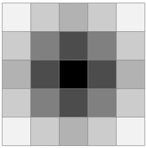
Figure 3.1 An illustration of a 5x5 grid. An example site is black shaded and its
neighbors are grey shaded. . . 18
Figure 3.2 A 5x5 grid model. Sites with same eignevector centrality have the
same degree of grey shading. . . 23
Figure 3.3 A star network. . . 28
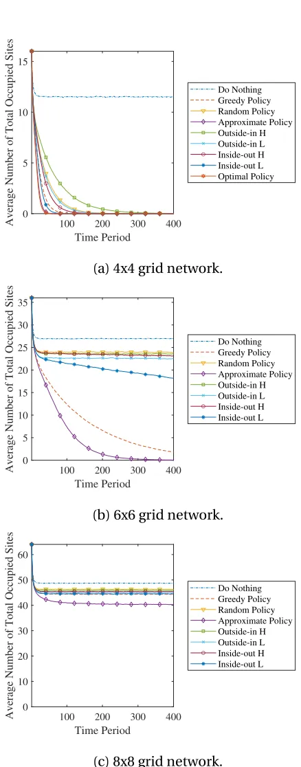
Figure 3.4 Time path simulations for a 4x4, 6x6 and 8x8 grid network where
actions is assumed to be partially effective (p0 =0,p1 =0.15,pn =
0.1,pt =0.7). The time paths represent an average over a ten
thou-sands replications. The gap between policies widens as the grid size increases. . . 34
Figure 3.5 Time path simulations for a 4x4, 6x6 and 8x8 grid network where
actions is assumed to be completely effective (p0=0,p1=0.15,pn=
0.1,pt =1). The time paths represent an average over a ten thousands
replications. The gap between policies widens as the grid size increases. 35
Figure 3.6 Time path simulations for 8x8 grid network where actions is assumed
to be completely effective, and spontaneous infection is set to small
non-zero value (p0=0.01,p1=0.15,pn=0.1,pt =1). The time paths
represent an average over a ten thousands replications. The results show that the system is likely to be recurrent. That is, the initial state
doesn’t affect the equilibrium level. . . 37
Figure 3.7 Sensitivity analysis of the spontaneous infection parameter(p0) for an
8x8 grid case. Other parameters are set to the baseline (p1=0.15,pn=
0.1,pt =1). The average is calculated over a ten thousands
replica-tions. Equilibrium levels increase asp0 increases. The initial state
appears to play an important role in the effectiveness of both the
outside-in and inside-out heuristic rules. . . 39
Figure 3.8 The standard deviation for the number of occupied sites. Model
pa-rameters values arep0=0,p1=0.15,pn=0.1,pt =1. The time paths
represent an average over a ten thousands replications. . . 41
Figure 3.9 An example 4x6 grid that illustrates the heuristic priority rule. It also
illustrates how sites are ordered in our simulation code. . . 43
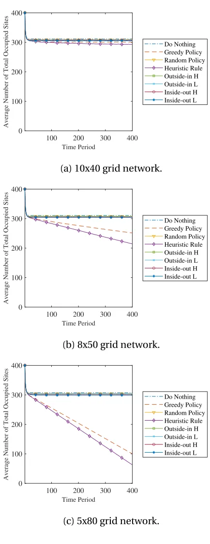
Figure 3.10 Time path simulations for a 5x80, 8x50 and 10x40 grid network where
actions is assumed to be completely effective (p0=0,p1=0.15,pn=
0.1,pt =1). The heuristic policy performance improves as the length
of the shorter side decreases. . . 44
Figure 3.11 An illustration of an 8x8 grid with clustered infected sites. Infected
Figure 3.12 Effect of clustered initial infestation in an 8x8 grid case. Parameters
are set to the baseline (p0=0,p1=0.15,pn=0.1,pt =1). The average
is calculated over a one thousand replications. Prioritization of the
small cluster results in a slightly better performance. . . 46
Figure 3.13 Time path simulations for a 20, 40, and 60 nodes star network (p0=
0,p1=0.1,pn=0,pt =0.7). . . 48
Figure 3.14 Chadès et al. (2011) test network. . . 50
Figure 3.15 The average number of occupied sites per period for a multi-layer
star network with 101 nodes (p0=0,p1=0.1,pn=0,pt =0.7). . . 51
Figure 4.1 Optimal Q-values at S=1 for different learning rates. The red dashed
line represents the optimal value at S=1, calculated using dynamic
programming. . . 62
Figure 4.2 Q-values for S=1 for each iteration using the optimal action according
to the Q-function using ten thousand simulated observations. . . 65
Figure 4.3 Box and whiskers plot of the percentage change of the second best
Q-values relative to the best for both the states where the model pre-dicts the optimal actions (correctly predicted) and the states where it predicts sub-optimal actions (incorrectly predicted). The whiskers length are 1.5 times the interquartile, which is the difference between the 75th and 25th percentiles values. The red pluses represent out-liers. It should be noted that the percentage change of the second best Q-values relative to the best for the correctly predicted states are
quite wide compared to the incorrectly predicted states. . . 68
Figure 4.4 Time path simulations for a 4x4, 6x6 and 8x8 grid network where
actions is assumed to be partially effective (p0 =0,p1 =0.15,pn =
0.1,pt =0.7). The time paths represent an average over a ten thousand
replications. . . 72
Figure 4.5 Time path simulations for a 4x4, 6x6 and 8x8 grid network where
actions is assumed to be completely effective (p0=0,p1=0.15,pn=
0.1,pt =1). The time paths represent an average over a ten thousand
replications. . . 73
Figure 4.6 Simulations results on Chadès et al. (2011) 101 nodes multi-layer star
network (p0=0,p1=0.1,pn=0,pt =0.7). . . 74
Figure A.1 Average number of occupied sites over ten thousands replications
and four hundreds periods for different policies for a 4x4 grid
sit-uation. The spontaneous infection parameter is set to zero (p0=0).
Figure A.2 Standard deviation of the number of occupied sites over ten thousand replications and four hundred periods for different policies for a 4x4 grid situation. The spontaneous infection parameter is set to zero
(p0=0). Action is assumed to be partially effective (pt=0.7). . . 86
Figure A.3 Average number of occupied sites over ten thousand replications and
four hundred periods for different policies for a 4x4 grid situation.
The spontaneous infection parameter is set to zero (p0=0). Action is
assumed to be completely effective (pt =1). . . 87
Figure A.4 Standard deviation of the number of occupied sites over ten thousand
replications and four hundred periods for different policies for a 4x4 grid situation. The spontaneous infection parameter is set to zero
(p0=0). Action is assumed to be completely effective (pt =1). . . 88
Figure A.5 Average number of occupied sites over ten thousand replications and
four hundred periods for different policies for a 6x6 grid situation.
The spontaneous infection parameter is set to zero (p0=0). Action is
assumed to be partially effective (pt =0.7). . . 89
Figure A.6 Standard deviation of the number of occupied sites over ten thousand
replications and four hundred periods for different policies for a 6x6 grid situation. The spontaneous infection parameter is set to zero
(p0=0). Action is assumed to be partially effective (pt=0.7). . . 90
Figure A.7 Average number of occupied sites over ten thousand replications and
four hundred periods for different policies for a 6x6 grid situation.
The spontaneous infection parameter is set to zero (p0=0). Action is
assumed to be completely effective (pt =1). . . 91
Figure A.8 Standard deviation of the number of occupied sites over ten thousand
replications and four hundred periods for different policies for a 6x6 grid situation. The spontaneous infection parameter is set to zero
(p0=0). Action is assumed to be completely effective (pt =1). . . 92
Figure A.9 Average number of occupied sites over ten thousand replications and
four hundred periods for different policies for a 8x8 grid situation.
The spontaneous infection parameter is set to zero (p0=0). Action is
assumed to be partially effective (pt =0.7). . . 93
Figure A.10 Standard deviation of the number of occupied sites over ten thousand replications and four hundred periods for different policies for a 8x8 grid situation. The spontaneous infection parameter is set to zero
(p0=0). Action is assumed to be partially effective (pt=0.7). . . 94
Figure A.11 Average number of occupied sites over ten thousand replications and four hundred periods for different policies for a 8x8 grid situation.
The spontaneous infection parameter is set to zero (p0=0). Action is
Figure A.12 Standard deviation of the number of occupied sites over ten thousand replications and four hundred periods for different policies for a 8x8 grid situation. The spontaneous infection parameter is set to zero
(p0=0). Action is assumed to be completely effective (pt =1). . . 96
Figure A.13 Average number of occupied sites over a thousand replications and four hundred periods for different policies for a 8x50 grid situation.
The spontaneous infection parameter is set to zero (p0=0). Action is
assumed to be partially effective (pt =0.7). . . 97
Figure A.14 Standard deviation of the number of occupied sites over a thousand replications and four hundred periods for different policies for a 8x50 grid situation. The spontaneous infection parameter is set to zero
(p0=0). Action is assumed to be partially effective (pt=0.7). . . 98
Figure A.15 Average number of occupied sites over a thousand replications and four hundred periods for different policies for a 8x50 grid situation.
The spontaneous infection parameter is set to zero (p0=0). Action is
assumed to be completely effective (pt =1). . . 99
Figure A.16 Standard deviation of the number of occupied sites over a thousand replications and four hundred periods for different policies for a 8x50 grid situation. The spontaneous infection parameter is set to zero
(p0=0). Action is assumed to be completely effective (pt =1). . . 100
Figure A.17 Average number of occupied sites for four hundred periods for dif-ferent policies for a multi-layer star network with 101 nodes. The
spontaneous infection parameter is set to zero (p0 = 0). Action is
assumed to be partially effective (pt =0.7). . . 101
Figure A.18 Standard deviation of the number of occupied sites over a thousand replications and four hundred periods for a multi-layer star network with 101 nodes. The spontaneous infection parameter is set to zero
(p0=0). Action is assumed to be partially effective (pt=0.7). . . 102
Figure A.19 Average number of occupied sites over a thousand replications and four hundred periods for different policies for a multi-layer star net-work with 101 nodes. The spontaneous infection parameter is set to
zero (p0=0). Action is assumed to be completely effective (pt=1). . 103
Figure A.20 Standard deviation of the number of occupied sites over a thousand replications and four hundred periods for a multi-layer star network with 101 nodes. The spontaneous infection parameter is set to zero
CHAPTER
1
INTRODUCTION
1.1
Introduction
This dissertation generally focuses on the problem of resource allocation over space and
time. We explore several approximate dynamic programming (ADP) methods (Powell 2008)
for controlling a stylized stochastic invasive species dynamic spatial model. We specifically
focus on the situation where the dimension of the problem is intractable to solve with exact
numerical methods, such as dynamic programming (Bellman 1954). Although our study
is based on a stylized invasive species problem, its implications could be useful for other
This chapter consists of two main parts: a literature review and a description of the
dissertation outline. The literature review starts with a discussion of the importance of the
spatial model models in economics, in general, and resource economics more specifically.
The review concludes with a discussion of the literature that has explored approximate
dynamic programming methods in resource economics problems.
1.2
Literature
Many fields of sciences use spatial models, including ecology and resource economics.
Disease spread (Ferguson et al. 2005), pest infestation (Bianchi et al. 2010), and invasive
species (Epanchin-Niell and Hastings 2010) are some examples. Spatial models can be
either implicit or explicit.
Explicit models are models that track the dynamics of the state of the locations
individ-ually. Bianchi et al. (2010) provides examples of such models. Implicit models are models
that track the dynamics of the state of the locations in a categorized aggregate way. Spatial
category count models are examples of implicit models (Fackler 2012). To illustrate the two
types of models, suppose we have several sites,n, where some pest can infest each of them.
Assume that the infestation level represents the state of each site. An explicit model in
this example tracks the evolution of the infestation level for each site, while for an implicit
model, we keep track of the evolution of the number of sites in each category of infestation
level (i.e., low, medium and high).
Spatial models have played an important role in economics for at least a century. For
example, Hotelling’s location model (Hotelling 1929) and the work by (Sraffa 1926) are
considered influential works in the theory of firms’ competition where space plays an
explicit dynamic models and considered a seminal work in the field of urban economics
and complexity economics (Arthur 1999). In relatively recent work, the spatial nature of
economics problem is contextualized in what is known as the New Economics Geography
(Krugman 1998).
In resource economics, space plays an important role. Albers et al. (2010) classifies
spatial resource economics studies into two types. The first is positive studies; that is, they
focus on studying the effect of policy changes on some economic outcomes. The second is
normative or resource management studies.
Positive resource economics studies branch into many categories. Hedonic valuation
models (Lancaster 1966; Court 1939; Waugh 1928), and sorting models (Palmquist 2005)
are some of the well-known branches where space matters (Ando and Baylis 2014).
Hedonic valuation models are based on the idea that product prices are derived from
their characteristics (Court 1939). An example is the valuation of housing attributes such as
proximity to open space, farmlands, wetlands, and other environmental and infrastructure
amenities (Johnston et al. 2002). Hedonic methods play an important role in resource
economics policies (Palmquist and Smith 2001). Taylor (2003) provides an overview of the
hedonic valuation approach.
Sorting models are used to study the equilibrium sorting behaviors of heterogeneous
agents taken into account the endogeneity of the sorting process (Kuminoff et al. 2010).
The work of Klaiber and Phaneuf (2010) is an example. They use sorting models to address
household location preference toward open spaces. Kuminoff et al. (2010) provides an
Space plays an essential role in many of the resource management problems. There are
two major approaches to dealing with spatial resource management problems. The first is
the dynamic optimization approach. The second is the heuristic policy approach (Chadès
et al. 2011).
The dynamic optimization approach is used to solve small tractable problems or to
get policy insights for larger problems (Epanchin-Niell and Wilen 2012). For example,
Sanchirico and Wilen (1999) studies the equilibrium nature of the dynamics of renewable
resources over space. The spatial nature in their model is manifested in the form of
inter-connected patches of habitats. Costello and Polasky (2004) explores the problem of reserve
site selection, where the objective is to maximize the number of conserved species over
a fixed planning horizon. Brock and Xepapadeas (2011) derives analytical results of the
steady-state spatial patterns due to human actions for biological processes.
Heuristic policy approach has been used in several resource economic problems with a
large dimension where dynamic optimization methods may not be tractable. For example,
Marcel Salathe (2010) develops an immunization policy and explores it in a social network
with community structure (M. Girvan and Newman 2002). Chadès et al. (2011) proposes
a rule of thumb to control the spread of invasive species over certain spatial network
structures. Perry et al. (2017) proposes a priority policy rule based on network centrality
measures to control invasive species over a spatial network structure.
There are a good number of studies of control problems for spatial models in both
biology and ecology that are very relevant to resource economics. Hof and Bevers (2002)
provides a comprehensive overview of the use of optimization and simulation models
in ecological economics applications. They also provide a discussion of why
simulation-based-optimizations has drawn less attention by resource economists. DeAngelis and Yurek
Spatial models can be seen, and modeled, as a network model, where a particular
connectivity structure connects sites. Chadès et al. (2011); Laber et al. (2018) are some
works that represented spatial structure in a network framework. There is a rich literature
in the network field that discusses dynamic processes over networks. Newman (2009) and
Lang et al. (2018) discuss the spread of a disease over a network. Liu et al. (2016) studies
immunization strategies in network structures. Proulx et al. (2005) provides an overview of
the network analysis for ecological applications, such as the spread of invasive species. The
works mentioned above are of resource economics nature. Newman (2007); Barabási (2016);
Strogatz (2001) provide general expositions to networks, including networks coupled with
dynamic processes.
The management and the control of invasive species, (Epanchin-Niell and Wilen 2012;
Chadès et al. 2011), is considered a critical and important problem. It has attracted the
attention of both ecologists and resource economists (Olson and Roy 2002).
Invasive species are estimated to cost more than a hundred billion dollars per year
(Olson and Roy 2002). The explicit spatial nature of invasive species management and the
uncertainty in the dynamics of the species are critical (Meier et al. 2014; Chalak et al. 2011).
Spatially explicit models suffer from the curse of dimensionality, that is they grow
exponen-tially in size with the number of sites. Efficient methods such as Dynamic Programming
(Bellman 1954) can only solve small size problems and is intractable for larger ones.
The research effort of explicit spatial modeling of the problem is quite limited
(Epanchin-Niell and Wilen 2012). Recent research concerned with relatively large dimensional explicit
invasive species spatial model is either based on deterministic models (Epanchin-Niell
and Wilen 2012) or development and testing of heuristic rules based on stochastic models
(Chadès et al. 2011; Perry et al. 2017).
approx-imate dynamic programming (ADP) methods (Powell 2011) in obtaining good policy rules
for stochastic dynamic spatial problems where dynamic programming is deemed infeasible.
We explore and apply some ADP methods to the invasive species stochastic spatial model
of Chadès et al. (2011). Our focus is more on the computational aspects of the methods,
in the sense of what works and what may not work. This distinguishes our research from
similar other researches, such as Epanchin-Niell and Wilen (2012), and Chadès et al. (2011).
The focus of Chadès et al. (2011) is on proposing a heuristic rule for a spatial stochastic
model. Epanchin-Niell and Wilen (2012) focuses on providing policy insights by solving a
deterministic larger dimensional spatial model using mixed-integer programming. Our
research provides insight into the potential of some approximate dynamic programming
methods.
In addition to that, we propose a simple-to-implement novel method. The method
exploits prior knowledge of the model, such as potential symmetry in the model, into the
structure of a policy rule. The method we propose utilizes some network measures. The use
of prior knowledge in function approximation has been shown to have a significant impact
on the efficiency of the function estimation (Belbute-Peres et al. 2018). We also illustrate
that the policy approximation method under our study can help in deriving simple heuristic
rules. Policymakers can apply such rules for problems with very large dimensions.
Economic research on the methods of approximate dynamic programming (ADP) is
largely based on solving small and moderate size problems (Judd et al. 2011). Springborn
and Faig (2019); Laber et al. (2018) are the only works we are aware of that explores ADP
methods for large dimensional resource management problems.
Springborn and Faig (2019) demonstrates ADP on a simple stochastic fishery problem
developed by Reed (1979). In their problem, they have one state variable, which is the stock,
based on approximating the value function using Gaussian process regression (Rasmussen
and Williams 2005).
Laber et al. (2018) work is based on the dynamic treatment regime methods (Murphy
2003). Their novel contribution is in extending it to a spatial situation where the number
of possible actions is very large. They demonstrate their method on the control of the
white-nose disease in bats.
Our work extends the literature of ADP in resource economics in multiple aspects. First,
we explore ADP methods that have not been explored in the mentioned works. Second, we
apply those ADP methods to a spatially explicit stochastic invasive species control problem.
Third, we show that some ADP methods, such as policy approximation methods, can help
in deriving simple heuristic rules that can be applied to very large dimensional problems.
1.3
Dissertation Outline
The dissertation consists of three main parts. The first part, which is the second chapter,
provides a general overview of Markov Decision Process (Bellman 1957), Dynamic
Pro-gramming (Bellman 1954), and Approximate Dynamic ProPro-gramming (Powell 2011). This
part aims to familiarize the reader with fundamental concepts that later chapters rely on.
Additionally, we provide a short introduction to the importance of approximate dynamic
programming methods and the difficulty associated with them.
The second part, which is the third chapter, presents the first method that we explore.
The method is based on policy function approximation, and the estimation method
pro-posed by Smith (1990) and explained in Judd (1998). The method also appears to be
in-dependently proposed by Moxnes (2003) in what he names as stochastic optimization in
Chadès et al. (2011).
The third part, which is the fourth chapter, discusses and explores some of the value
function approximation methods. Our treatment, in this part, has two objectives. The
first is to provide an overview of reinforcement learning (Watkins 1989; Sutton and Barto
2018), which is a different terminology of approximate dynamic programming in computer
science. The second is to illustrate and explore the method of Least-Square-Policy-Iteration
CHAPTER
2
PRELIMINARIES
2.1
Introduction
This chapter provides an overview of some fundamental methods and concepts that are
useful for subsequent chapters. The treatment of this chapter will be as follows. First,
we introduce the Markov decision process (MDP) as a framework for modeling dynamic
decision-making problems. Second, we introduce an overview of dynamic programming
(DP) and Bellman equation (Bellman 1954). Third, we provide an overview of the two
widely used dynamic programming solution methods: the value function iteration, and the
approximate dynamic programming (ADP) (Powell 2008).
2.2
Markov Decision Process
A Markov decision process (MDP) (Bellman 1957; Howard 1960) consists of a set of state and
action variables, a reward function, and a transition rule that models the evolution of the
state variables for each action. In the MDP, future states depend only on current states, and
actions (i.e., history is irrelevant). MDP provides an elegant framework for modeling many
practical dynamic decision-making problems of stochastic nature (Howard 1960). Dynamic
programming (Bellman 1954) is considered an efficient tool for solving MDP problems
(Howard 1960; Bellman 1957). Resource economics is pervasive with such MDP problems
where agents, such as resource managers, are in a situation where they seek to take the
best actions over some period of time in order to achieve certain goals. Such situations, or
problems, are formulated as dynamic optimization problems (Marescot et al. 2013).
2.3
Dynamic Programming
Any dynamic optimization problem generally consists of two main components (Puterman
1994): a system model, and an objective function. The system model is a model that
de-scribes how the system behaves, and it consists of three main components: state variables,
which describe the state of the system, action variables, which describe the actions that can
be taken on the system, and a transition model, which describes how the system evolves.
To state this in a mathematical form and assuming all the variables are discrete, let
St represent a vector of state variables,At a vector of action variables, andεt represents
infinite horizon problem, we uset to represent the current period andt +1 for the next
period. LetSt+1=g(St,At,εt)represents the system model, which can be stochastic, and
r(St,At)represents a reward function. A widely used objective function is the expected
discounted sum of the reward function over some time horizonT (Marescot et al. 2013;
Puterman 1994). Let β be a discount factor. An agent’s problem is to seek the optimal
actions that maximize the expected discounted rewards given the current state (S1). That is
max At
T X
t=1 βt
E[r(St,At)|S1] (2.1)
such that (2.2)
St+1=g(St,At,εt). (2.3)
There are several ways to solve such a problem. If the problem is an MDP, which is
the case for the model under our study, then dynamic programming, (Bellman 1954), is
considered an efficient and elegant way to solve such a problem (Bellman 1957). Letπ
denote a policy function, which is a mapping from the states to the actions, and letV(St)
be the value function atSt, which is the expected discounted sum of rewards following a
policyπ. The above optimization problem can be written in a recursive form, in what is
known as the Bellman equation, as
V(St) =max
At
r(St,At) +βE[V(St+1)|St,At]. (2.4)
Bellman equation can be solved in different ways, as illustrated in the subsequent
sections. The solution is characterized by an optimal policy function, let it beπ∗
t(St), which
gives the optimal action given stateSt, and an optimal value function, let it beVt∗(St). For
time-independent).
2.4
Value Function Iteration
The Bellman equation is of recursive form. The value function iteration method (Bellman
1957) states that the infinite recurrence of the Bellman equation results in the maximum
value function. To illustrate this, letV∗denotes the vector of maximum values for every
state,V0denotes a vector of initial values, which could be set arbitrarily to zero, andVn be
the vector of values at iterationn. Starting withn =0, then value function iteration method
solves:
Vn+1(St) =max
At
r(St,At) +βE Vn(St+1), (2.5)
until|Vn+1−Vn|< ε, whereεis some small number. Given certain conditions (Puterman
1994),Vn approachesV∗for large n, that is lim
n→∞Vn=V∗. For finite horizon problems,
one would start with the last period values and substitute backward into the Bellman
equation.
2.5
Policy Iteration
Howard (1960) proposed the policy iteration algorithm to solve infinite horizon problems.
The algorithm consists of two steps. The first is to improve the policy by using the most
recent values of the value function. That is, in iterationn,
πn=argmax
π r(St,At) +βE V n(S
The second step is to update the values of the value function given the new policy. That is
Vπn(St) =r(St,πn(St)) +βE Vπn(St+1). (2.7)
Equation (2.7) is a system of linear equations that can be solved for the value function at
each state. LetPπn denote the transition matrix, where columns represents current state
and rows future states for policyπn, thenE Vn(St+1) =Pπn
0
Vn(S
t+1), and Equation (2.7) can
be written as
Vπn =r(S,πn(S)) +βPπn
0
Vπn (2.8)
=⇒Vπn = (I −βPπn0)−1r(S,πn(S)). (2.9)
Note that we have dropped the time scripts since we are assuming an infinite horizon and
henceVπn is stationary (Howard 1960).
The policy iteration method distinguishes itself from the value function iteration method
in two aspects (Howard 1960). First, it converges when no policy improvement occurs in
two consecutive iterations. Second, it tends to converge in fewer iterations.
2.6
Approximate Dynamic Programming
Although dynamic programming is a powerful method for solving dynamic optimization
problems, it suffers from the curse of dimensionality. Powell (2011) explains this as three
curses of dimensionality. The first one is related to the state space, which is all possible
as it grows exponentially with the number of state variables. The second one is related
to the action space, which is all possible actions that can be taken. Similarly, the action
space grows exponentially with the number of action variables. The third one is related to
the stochasticity of the system, or the outcome (random) variables (i.e.,ε). The outcome
space increases exponentially with outcome variables making the computation of the
expectation hard or even impossible. This makes dynamic programming intractable for
large dimensional problems, and hence approximate dynamic programming methods
come into play.
Approximate dynamic programming (ADP) is a collection of different methodologies
that aims at obtaining a near-optimal policy or value function (Powell 2008). Most methods
are based on approximating either the policy function or the value function by some
parametric or non-parametric functions (Powell 2011). Approximate dynamic programming
is also known by other names, such as neurodynamic programming (NP) (Bertsekas and
Tsitsiklis 1996) and reinforcement learning (RL) (Sutton and Barto 1998). The success
of approximate dynamic programming methods is problem specific (Powell 2011). This
means a method that works for a particular type of problem may not work for other types of
problems. This requires an exploration of a variety of methods for the problem of interest.
For example, a method based on policy function approximation may work better for certain
problems, while a method based on value function approximation may work better on
others.
In our research, we aim to explore and apply different methods on a stylized spatial
invasive species MDP problem. The stylized model is based on Chadès et al. (2011)
stochas-tic discrete susceptible infected susceptible (SIS) diffusion, or transmission, model. Our
CHAPTER
3
A RANK BASED POLICY FUNCTION
APPROXIMATION IN SPATIAL MODEL
3.1
Introduction
This chapter aims at introducing and testing the performance of a simple tunable
approxi-mate policy function. The discussion in this chapter will be as follows. In the first part, we
provide a brief review of stochastic optimization in policy space as an approximate dynamic
programming method (Moxnes 2003; Judd 1998; Smith 1990). The second part lays out
opti-mization method followed by a discussion of our approximate policy function. Afterward,
we provide an overview of how features of the policy function can be selected. Next, we
discuss the different types of approximate dynamic programming evaluation methods. The
last part is the analysis part, which explores our rank-based policy on both regular grids
situation as well as Chadès et al. (2011) multi-layer test network.
3.2
Policy Function Approximation
As we have mentioned in previous chapters, approximate dynamic programming is a
collection of different types of methodologies that aim at obtaining a near-optimal policy
or value function. One simple method is parametric policy function approximation. As
explained in Judd (1998) and Smith (1990), one would first propose a parametric function
for the policy rule, and then estimate the parameters through simulation, such that the
objective function is maximized.
To illustrate the method, letAt =π(S,α)be a parametric policy function approximation,
whereαis a vector of parameters. LetM denote the number of simulation replications of
the system model over timeT 1. The optimization problem can be solved by solving for the
vector of parameters (α)in
max
α
1 M
M X
m=1 T X
t=0 βt
r(Sm t,π(Sm t,α)). (3.1)
There are many optimization techniques, or solvers, that can be used to solve the
problem in Eq. (3.1). The choice of the solver to be used depends on the continuity and
linearity of the objective function (Eq. 3.1). As we show in later sections, in our spatial
1Note that we have to chooseT large enough such that the solution is close enough to the infinite horizon
problems, both the reward and policy functions are discrete. Additionally, our proposed
policy function will be non-linear. Thus, we use a robust gradient-free global optimizer
such as DIvided RECTangles (DIRECT) optimization algorithms.
Define a feature as a function of state variables that can be used as a predictor in the
policy function. The choice of features in the approximate policy function is one significant
and critical thing to be considered to obtain a good policy function. It is a very challenging
step and is based on both trial and error and the consideration of the structure of the
problem.
Once some features are decided on, it is essential to know how good or how close
is the approximate policy to the optimal one or some baseline policies. Evaluating the
performance of the approximate function is another major challenge. Powell (2008) states
three ways for policy evaluation. The first one is to compare the approximate policy to an
optimal policy of a simpler problem. The second is to compare it to an optimal policy of a
deterministic version of the problem. The third way is to compare it to a myopic or greedy
3.3
Model
Figure 3.1: An illustration of a 5x5 grid. An example site is black shaded and its neighbors
are grey shaded.
Our analysis is based on Chadès et al. (2011) model. We explore both regular grid model
and Chadès et al. (2011) multi-layer star network model. In both situations the model
consists of multiple sites numbered from 1 toNs. Each site is represented by a state variable,
Si, that takes two values: 1: site occupied, and 0: site unoccupied. We assume that one site
is treated each period, and the action variable represents the number of that site and 0 if
no action is to be taken. We also assume that preventive action (treating an uninfected site)
is possible. LetSi denote the state variable for a sitei,Athe action variable, which is the
site to treat, andSi+the next period state value. GivenSi, andA, the state variable of sitei
evolves to the occupied state according to the probability model:
P(Si+=1|Si,A) =Si(1−1A=i)(1−pn)+Si1A=i(1−pt)+(1−Si)(1−1A=i)[1−(1−p0)(1−p1)qi], (3.2)
no action is taken,(1−pt)is the probability that sitei will remain occupied in the next
period when an action is taken,[1−(1−p0)(1−p1)qi]is the probability that sitei becomes
occupied when no action is taken due to having occupied untreated neighbors ((1−p1)qi)
or due to spontaneous or exogenous occupation (1−p0) whereqi is the number of directly
connected sites (neighbors) to sitei that are occupied but not treated. The model also
assumes that unoccupied treated sites remain unoccupied. The neighbors of a site are
defined to be the four directly adjacent neighbors to sitei, which is known as the von
Neumann neighborhood. Figure 3.1 shows an illustration of a five by five grid, where each
cell is a site. An example site is black shaded, and its neighbors are grey shaded.
Now we define the management problem. Letπ(St,α)denote a policy rule which maps
state to action at periodt whereSt is ann-element vector that represents the state values
of the sites at timet, andαis a vector of parameters. The management problem can be
characterized by the policy ruleπ(St,α∗)that achieves the minimum expected discounted
sum of the number of occupied sites, that is
min
α E
T
X
t=0 βt
n X
i=1 Si t|π
, (3.3)
whereβis a discount factor, andT is the terminal period. In our analysis, we assume that
the time horizon is infinite, where we approximate it by finite time horizon ofT periods.
3.4
Policy Rule
The functional form of our tunable or parametric policy rule can generally be expressed as
follows:
Si t e I n d e xi=φ(S,αi), (3.4)
whereS is a vector of the states variables,φis a function, which can be linear or non-linear,
andαi is vector of parameters to be estimated for sitei. The action to be taken is
A=π(S,α) =argmax
i (
Si t e I n d e xi), (3.5)
that is an action will be taken for the site with the largest index value. It should be noted
that the policy rule is non-linear inα. The non-linearity is due to the max operator, even if
the site index (φ) is linear inα.
3.5
Features Selection For Spatial Models
As stated previously, feature selection is one challenging step in the construction of
approx-imate policy rules. In spatial models, one natural feature is the state of the site itself. That
is, our proposed policy rule can be stated asSi t e I n d e xi=αi·Si. Although such a simple
policy might result in near-optimal policy rules in small problems, it may not be sufficient
for larger problems. This requires one to add features that could be functions of the states
of other sites. Representing the spatial structure of the model efficiently is very important
and helps in the construction of features.
One simple, yet powerful, way to represent a spatial model is to represent it by, what
adjacency matrix is a symmetric matrix where each row represents a sitei, and each cell in
rowi, and columnj contains "1" if sitei is connected (neighbor) to sitejand "0" otherwise.
There are two advantages of using the adjacency matrix. First, it allows exploiting the
graph and network theory literature in the construction of features. Second, it allows us
to calculate the features in an efficient way, which is very critical in simulation-based
optimization as the policy rule is called many times.
To illustrate this, suppose we have a two by two grid model. The model can be
repre-sented by the adjacency matrix
ζ=
0 1 1 0
1 0 0 1
1 0 0 1
0 1 1 0
. (3.6)
Suppose that we plan to add a new feature to the policy rule, such as the total number of
neighboring sites with state valuesSi=1, and denote it byqi. The feature can be efficiently
calculated asqi=ζ·Swhere S is a column vector of the state values.
3.5.1
Network Centrality
In this section, we discuss how network measures, such as network centrality can be used to
construct useful features. Centrality measures define how important a node is in a network
(Newman 2007). The simplest centrality measure is known as the degree centrality. The
degree centrality for a node (or a site) in a network is defined to be the number of directly
connected nodes to that node. For example, under this definition, a node that is directly
that is directly connected to less number of nodes.
The degree centrality does not reflect a deep measure of centrality for a node (Newman
2007). For example, one could have two types of nodes, one that has a large number of
neighbors, hence has large degree centrality, but its neighbors have no other neighbors,
and another node that is connected to few neighbors, hence has a small degree of centrality,
but its neighbors have a large number of neighbors. Based on degree centrality, one would
conclude that the first node is more central than the second. Furthermore, in the grid
networks, the degree centrality will be the same, that is four, for all interior sites that are
one site away from the edges, and hence will not be a good measure of the position of the
sites relative to the edges.
Eigenvector centrality is a centrality measure that is deeper than degree centrality in the
sense that it considers not only the directly connected neighbors but also the neighbors of
the neighbors. This centrality measure provides a score of how central a node is (Newman
2007).
Following the treatment in Newman (2007) and Bonacich (1972), letxirepresent the
eigenvector centrality of nodei andζan adjacency matrix for the network of interest, then
the eigenvector centrality for nodei is defined as2
xi=
1
λ X
j∈Gi
ζi jxj, (3.7)
or in vector form as
λx=ζ·x (3.8)
wherex= [x1,x2, ...,xn], andGiis the set of neighbors for nodei. The eigenvector centrality
is the vector associated with the largest eigenvalue for the adjacency matrixζ.
Eigenvector centrality can also be used in parameter dimension reduction of a policy
function. We illustrate this by an example. Suppose we have a five by five regular grid, as
shown in Fig. 3.2. Looking at the figure, one can observe six types of locations as
distin-guished by their eigenvector centrality. In a policy function, one can utilize this symmetry
by assuming each type of site has a different set of parameters to be estimated instead of one
for each site, which would result in a significant reduction in the dimension of parameters
to be estimated. For example, suppose we have a policy function with one parameter for
each site, then we would have a total of 25 parameters. If we constrained the parameters to
be the same for each site type, then this would reduce the number to 6 parameters.
Figure 3.2: A 5x5 grid model. Sites with same eignevector centrality have the same degree
3.6
Issues and Challenges
There are several issues and challenges of the rank-based policy rule, as stated in Eq. (3.5)
and the estimation method in Eq. (3.1). The first one is that the policy rule suffers from
the identification issue. The Identification issue is a result of the ordinal nature of the
policy rule. To illustrate this, and given a specific stateS, let j denote the index of the
site with the maximum value ofφ as calculated in Eq. (3.4). For any δsuch that |δ| <
m i n(φj −φi)∀i, perturbation of the values ofφi byδwill still preserve the rank of sitej
being the maximum. Additionally, given fixed values ofφi, the vector ofαi for each sitei is,
generally, non-identified. The identification issue should not be deterrent from using such
a policy rule. Some widely and successfully used function approximation methods, such as
neural networks, suffer from such an issue (Albertini and Sontag 1993). Solving or reducing
the severity of it, however, may improve the efficiency of the estimation process.
In certain problems, there could be redundancy in the parameters that contribute to the
identification issue. This is the case in our regular grid situation, where the spatial structure
is symmetric. We can resolve this redundancy by constraining the sites that have the same
eigenvector centralities to have the same parameters, as illustrated in the previous section.
The specification of the policy rule in Eq. (3.5) does not illustrate how ties could be
broken-up. In other words, in case two sites have the same values ofφ, which site do we
choose? One way is to break the ties by choosing a site randomly. Another way is to choose
the one that appears first in the list of sites ranks. For computational convenience and
efficiency, we choose the second away.
Our simulation-based estimation approach requires setting certain hyper-parameters
such as the number of replications and the time horizon. We choose the number of
estimation stage, where we use simulation to estimate the parameters of the policy rule, we
set it to a hundred replications. In the evaluation stage, we set the number of replications
to ten thousand in order to make the simulated time paths smoother. In all our analyses,
we use the simulation-based expected number of occupied sites at each time period over
the number of replications as our policy performance measure. We use fewer replications
in the estimation stage than the evaluation stage as it is very computationally intensive
since the optimizer calls our simulator thousands of times.
The other thing to decide on is the time horizon. Note that we can express the infinite
horizon value function (V∞)following a policyπas
V∞π =
∞
X
t=0
βtE Rπ
t ≈
T X
t=0
βtE Rπ
t +β
T+1
∞
X
t=0
βtR˜π= T X
t=0
βtE Rπ
t +
βT+1R˜π
1−β , (3.9)
whereRtπis the reward at timet following policyπand ˜Rπis the expected equilibrium level
following policyπ. The time horizon (T) is chosen, such that the second term in (3.9) is
3.7
Policy Evaluation
In order to test or explore the performance of our proposed policy function, we need to use
some evaluation methods. The literature seems to lack a thorough treatment of evaluation
methodologies for approximate dynamic programming methods. Nevertheless, Powell
(2008) states three methods where some or all may apply to the problem of interest.
The first method is to compare the policy obtained using the approximate dynamic
programming methods, such as the stochastic optimization in policy space, with optimal
policy for a simplified or smaller version of the problem. For example, in a spatial model,
we can compare the policy rule obtained using approximate methods with the optimal rule
by solving a problem with a number of sites up to a level where it can be solved optimally.
The second method is to solve a deterministic version of the problem optimally and
to use approximate methods and compare those two policies. In some problems, the
deterministic version of the problem allows one to solve a larger problem using other
optimization methods.
The third method is to compare the approximate policy rule with a myopic or greedy
rule. For example, in our spatial model, the myopic rule is to take action on the site that
minimizes the expected next period damages.
In our analysis, we apply the first and third evaluation methods but not the second one.
We avoid the second one as there does not seem to be an obvious way to get a deterministic
version of the model without making some critical assumptions. For example, in our model,
the diffusion of pests to a site depends on its infected neighbors in a probabilistic way, that
is the higher the number of infected neighbors, the higher is the probability of that site to
be infected next period. If we are to make this part of the model deterministic, then we
neighbors exceeds the threshold. This is tricky and may result in misleading conclusions
on how the policy might do in the stochastic situation. Another difficulty is that the way
we would be able to solve a larger version of our deterministic model is through integer
programming (Epanchin-Niell and Wilen 2012), which means that the solution obtained
will be defined as a sequence of actions for every period. It is not apparent how would one
convert this, if even possible, to a policy function that is defined for every possible state.
3.8
Analysis
We will start our analysis with an extreme network of four isolated sites. This aims to
familiarize the reader with the idea of this research and the methodology. Additionally, we
use it to illustrate some concepts.
Next, we aim at exploring the performance of our approximate policy for larger networks.
We will explore both regular grid networks and Chadès et al. (2011) multi-layer star network.
The objective of this exploration is to seek answers to several main questions. The first is
whether the stochastic optimization method with our non-linear policy function would
work or not. By this, we mean that even if the approximate policy has a correct functional
form in the sense that it could result in the optimal policy, the optimization method may or
may not result in good estimates of the parameters. In analogy to a simple linear regression
model, suppose we know the correct model or the data generation process. If we do not use
a good estimation method (i.e., OLS), then we may not get a good estimate of our correctly
specified model. The second point is that if it works, then how good is it compared to other
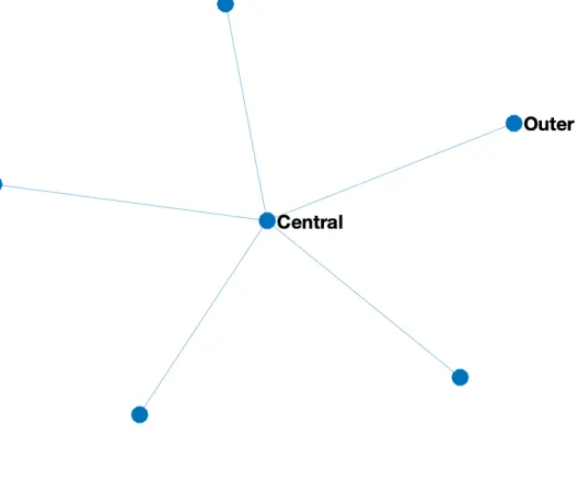
Figure 3.3: A star network.
To be able to answer those questions, we need to define features for the policy rule in
Eq. (3.5), and define baseline comparison policy rules. The features that we will use in the
policy rule are the state of the site itself, and the number of infected neighbors interacted
with the state of the site. That is
Si t e I n d e xi=α1i·S1i+α2i·S1i·qi, (3.10)
whereqi is the number of infected neighbors. We selected those features as they generalize
(Chadès et al. 2011). Additionally, we believe that the rule also generalizes the Chadès et al.
(2011) rule of thumb. We illustrate this on the star network mentioned in Chadès et al. (2011)
and shown in Fig. 3.3. An inside-out rule prioritizes the treatment of the central node over
the outer nodes, that is central node is treated first. Leti represents the outer nodes, and j
represents the central node, then to implement the inside-out using our rule, we can set
α1i,α1j andα2ito 1 andα2j to 1+a small number. The outside-in rule does the opposite:
which is to treat the outer nodes first, then the central ones. This can be implemented by
settingα2ito -1 andα2j to -1- a small number, while settingα1i andα1j to 1. Chadès et al.
(2011) rule of thumb treat half the outer nodes first then the central node then continuing
treating the rest of the outer nodes. To implement it we can setα1ito 1α1j to 3 , andα2i
andα2j to -1.
We will be using four policy rules for comparison. The first one is the optimal policy,
and this will only be used in the largest problem that can be solved optimally, which is the
four by four grid problem. The second is the myopic or greedy policy, which is to treat the
site that would minimize the expected damages in the next period. Mathematically, the
greedy policy is
G r e e d y(S) =min
A E
Xn
i
(Si+)|A,S
=min A
n X
i
Si+·P(Si+=1|S,A), (3.11)
whereSis a vector of the state of each site,Siis the state of sitei,Ais an integer number that
represents the site to be treated. The third rule is an inside-out rule, where the most central
site, according to the eigenvector centrality, is treated first. The fourth is the outside-in
rule, where the least central site is treated first. We will use two variations of the third and
the fourth rules. The first prioritizes the treatment to the site with the highest number
infected neighbors. The third and fourth policy rules are special cases of the policy in Eq.
(3.5) where we set the coefficients at certain values, as has been illustrated in the previous
paragraphs.
It should be noted that in our analysis, we assume that cost is irrelevant as we assume
that only one action per period is allowed. The one action per period assumption allows us
to solve the problem optimally, for comparison purposes, for a relatively larger number of
sites (about 16 sites). Model baseline parameters are shown in Table 3.1. In all our analyses,
we use the expected number of occupied sites (i.e., the damage) per period as a measure
of the performance of the policies. The default initial state for our simulations is the state
where all sites are being occupied. We will explicitly state the initial states for other cases
that we explore as well.
Table 3.1: Baseline and adjusted model parameters.
Parameter Base values
p0 0
p1 0.15
pn 0.1
pt 0.7,1
β 0.95
3.8.1
Isolated Network
To do a basic check of the proposed solution method and to illustrate and make some points
more concrete, we start by solving a simple and trivial problem. The problem consists of
four isolated sites with the setup mentioned previously, and the model parameters are set
according to the base values in Table 3.1.
This problem is trivial as a preventive action, which treats a site in order to prevent
the spread of infection, plays no role. This is because sites are isolated from each other,
and hence an optimal solution is trivial, which is to treat one of the occupied sites at each
period.
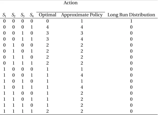
We solve this problem both optimally and using the approximate policy. There are
several points to illustrate. First, looking at Table 3.2, we can see that both the optimal and
the approximate policy solution give what we expect, which is to treat an infected site.
It should be noted that the approximate policy does not seem to break ties in the order,
as mentioned in the previous section. The reason for this is that, although one expects ties
for states that have more than one infected site, the coefficients of the approximate policies,
as shown in Table 3.3, for some sites are different, resulting in no ties in the rank for some
states. This also illustrates the identification issue in our policy rule.
Second, if we look at the long-run distribution in Table 3.2, computed using the
pre-sented optimal solutions, we see that complete eradication is certain. This means, in the
long run, and under the optimal policy, most states are never visited. It should be noted that
eradication is certain since spontaneous infection is ruled out in our setup. This necessitates
that we start with some sites being infected in the estimation of the approximate policy.
If we do not do so and alternatively started the simulation with all sites being uninfected,
the objective function, as in Eq. (3.3), will be the same for any parametric values, which is
zero.
Table 3.2: Policy rule: optimal versus approximate policy.
Action
S1 S2 S3 S4 Optimal Approximate Policy Long Run Distribution
0 0 0 0 0 1 1
0 0 0 1 4 4 0
0 0 1 0 3 3 0
0 0 1 1 3 4 0
0 1 0 0 2 2 0
0 1 0 1 2 2 0
0 1 1 0 2 2 0
0 1 1 1 2 2 0
1 0 0 0 1 1 0
1 0 0 1 1 4 0
1 0 1 0 1 1 0
1 0 1 1 1 4 0
1 1 0 0 1 2 0
1 1 0 1 1 2 0
1 1 1 0 1 2 0
1 1 1 1 2 2 0
Table 3.3: Estimated coefficients of the policy in Eq. 3.10 It should be noted that we have
infinite solutions (i.e., any positive coefficients result in the same policy).
Coefficient S1 S2 S3 S4
α1 0.4444 0.6667 0.4444 0.6667
3.8.2
Grid Networks
In this section, we analyze the policy rule in Eq. (3.10) on three regular grid networks: 4x4,
6x6, and 8x8. We constraint the coefficients of the policy rule for the sites with the same
eigenvector centrality measures to be the same as described in the previous section. We
analyze the policy rule in two versions of the system model. The first assumes that action is
partially effective , that ispt =0.7, while the other assumes that action is perfectly effective
pt =1.
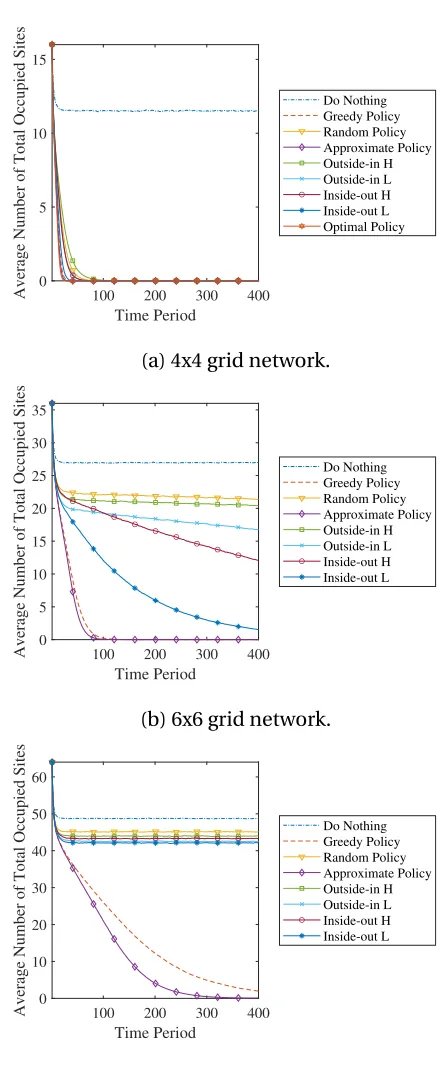
Looking at Figs. 3.4 and 3.5, we find that the approximate policy generally does well
compared to other policies, which suggests that the simulation-based estimation works for
our non-linear policy rule. As the size of the network increases, the gap increases between
the approximate policy and the greedy policy.
By constraining the number of coefficients to be estimated using the eigenvector
cen-trality, we significantly reduce the dimension of the policy function, and hence the burden
on the optimizer. The difference between the dimensions of the constrained and
uncon-strained policy functions for different grid sizes is illustrated in Table 3.4.
Table 3.4: Dimension of the constrained and unconstrained policy functions for different
grid sizes. Exploiting spatial symmetry in the problem by using eigenvector centrality
significantly reduces the number of parameters to be estimated.
Grid Size Policy Function Dimension
Unconstrained Constrained
4x4 32 6
6x6 72 12
100 200 300 400 Time Period 0 5 10 15
Average Number of Total Occupied Sites
Do Nothing Greedy Policy Random Policy Approximate Policy Outside-in H Outside-in L Inside-out H Inside-out L Optimal Policy
(a) 4x4 grid network.
100 200 300 400
Time Period 0 5 10 15 20 25 30 35
Average Number of Total Occupied Sites
Do Nothing Greedy Policy Random Policy Approximate Policy Outside-in H Outside-in L Inside-out H Inside-out L
(b) 6x6 grid network.
100 200 300 400
Time Period 0 10 20 30 40 50 60
Average Number of Total Occupied Sites
Do Nothing Greedy Policy Random Policy Approximate Policy Outside-in H Outside-in L Inside-out H Inside-out L
(c) 8x8 grid network.
Figure 3.4: Time path simulations for a 4x4, 6x6 and 8x8 grid network where actions is
100 200 300 400 Time Period 0 5 10 15
Average Number of Total Occupied Sites
Do Nothing Greedy Policy Random Policy Approximate Policy Outside-in H Outside-in L Inside-out H Inside-out L Optimal Policy
(a) 4x4 grid network.
100 200 300 400
Time Period 0 5 10 15 20 25 30 35
Average Number of Total Occupied Sites
Do Nothing Greedy Policy Random Policy Approximate Policy Outside-in H Outside-in L Inside-out H Inside-out L
(b) 6x6 grid network.
100 200 300 400
Time Period 0 10 20 30 40 50 60
Average Number of Total Occupied Sites
Do Nothing Greedy Policy Random Policy Approximate Policy Outside-in H Outside-in L Inside-out H Inside-out L
(c) 8x8 grid network.
Figure 3.5: Time path simulations for a 4x4, 6x6 and 8x8 grid network where actions is