Forward Kinematics and Differential Motion
Analysis of SCORBOT ER-V plus Robotic
System
Faijubhai R.Malek
Assistant Professor, Dept of Mechanical Engineering, G.H.Patel College of Engineering and Technology,
VallabhVidya Nagar, Gujarat, India
ABSTRACT: In this paper forward kinematic analysis and differential motion analysis of the SCOROT ER V-plus robotic system, which is a 5 d.o.f articulated robotic manipulator, following a specified trajectory is reported. Forward kinematic analysis uses D-H formulation and Differential motion uses Jacobians and determines angular positions and end-effector‟s translational and angular velocity at each via point of its trajectory in the Cartesian space co-ordinates respectively. A trajectory passing through initial point, lift off point, set down point and final point is interpolated in the joint space using cubic splines. The trajectory scheme assumes two more intermediate points on trajectory. Thus, there are five segments of the entire trajectory. A MATLAB source code is developed to obtain all the kinematics parameters and important conclusions are reported from the values obtained.
KEYWORDS:Robot, Forward Kinematics, Jacobians, D-H matrix, Trajectory.Introduction.
Nomenclature
Ve is a (6 x 1) vector of end-effector‟s translational and angular velocity with respect to fixed base
J(q) is a (6 x n) matrix known as a jacobian matrix relative to fixed base
.
q
is a (n x 1) vector representing rotational velocities of various joints of robot n is a number showing degrees of freedom of the roboti-1
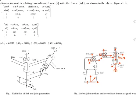
Ti a transformation matrix relating co-ordinate frame {i} with the frame {i-1}
5j jacobian matrix relative to the tool frame {5}
I. INTRODUCTION
The motion of an industrial robot manipulator is generally specified either in terms of the motion of various joints of the manipulator or that of the end-effectors in the Cartesian space. An accurate direct measurement of end-effector‟s position is a complex task and the implementation of a motion control system in Cartesian space can be very difficult.
Thus, in practice motion of various joints is converted in the end-effectors motion using forward kinematics. Kinematic parameters are necessary to consider in design and specifications planning, in trajectory planning
(programming), and in dynamic computations. A common feature of many of the application problems is the fact that the position of the arm end (end effectors) is frequently described by the user in Cartesian world coordinates [9].
However, control of link motions is achieved through driving and measuring (for the feedback purposes) of joint coordinates. If the kinematic parameters of the end effectors are expressed in terms of joint parameters, the transformation is called direct or forward kinematics.
As a rule, the end-effectors of a robot is programmed to follow a set of desired positions and orientations in the Cartesian space. When it is required to determine how each infinitesimal joint motion affects the infinitesimal motion of the manipulator end-effectors, one has to develop a mapping scheme between the joint motion and the corresponding end-effector‟s motion. This mapping is defined by a jacobian.
The forward kinematics at the differential level can be represented by a linear system, .
) (q q J
Ve ; (01)
Thus, determination of the end-effectors velocity vector involves determination of the jacobian matrix of the robot. As it can be seen from above given relation (01), jacobian is a function of a set of joint angles. „q‟ in turn determines the pose of the robot arm.
II. MATERIAL AND METHOD
Forward kinematics using D-H parameters:
A numerical procedure for deriving a transformation matrix relating two consecutive joints of a robot is discussed below.
A transformation matrix relating co-ordinate frame {i} with the frame {i-1}, as shown in the above figure-1 is:
1 0
0 0
cos sin
0
sin sin
cos cos
cos sin
cos sin
sin cos sin cos
1
i i
i
i i i i i i i
i i i i i i i
i i
d a a
T
(02)
1 0 0
0
0 i i i
i i i i i i i
i i i i i i i
d c s
s a s c c c s
c a s s c s c
(03) Where ci = cosi ; si = sini ; ci =cosi ; si =sini
Fig. 3 Co-ordinate axes assignment to each joint of SCORBOT in its home position
Fig. 4 Coordinate axes assignment to each joint of SCORBOT in its vertical position
Figure-3 represents assignment of coordinate axes to each joint of the robotic manipulator under consideration in its home position. Figure-4 represents assignment of coordinate axes to each joint of the robotic manipulator under consideration in its arm vertical position. At this stage it is important to take note that the coordinate axes assignment as shown in Figure-3 and 4 is not unique. There are several possible configurations for coordinate system definition.
Now, based on the above shown co-ordinate axes assignment scheme we have Denavit-Hartenberg kinematic parameters as given in table-1:
Table-1: D-H parameters for SCORBOT ER-Vplus
Where
a1=0.025 m ; a2=0.220 m ; a3=0.220 m ; d1=0.364 m; d5=0.100 m
Using above given kinematic parameters [8] and equation-2 the transformation matrices relating two consecutive frames i.e 0 T1,
1
T2 , 2
T3, 3
T4, and 4
T5 ; (04)
are obtained.
Now, the transformation matrix-relating frame {5} with the base frame {0} is given by:
0T5 =0T11T2 ……..4T5 ; (05)
1 0
0 0
) (
) (
) (
1 2 2 23 3 234 5 234
5 234 5
234
1 2 2 23 3 234 5 1 234 1 5 1 5 234 1 5 1 5 234 1
1 2 2 23 3 234 5 1 234 1 5 1 5 234 1 5 1 5 234 1 5 0
d s a s a c d c
s s c
s
a c a s a c d s s s c c s c s s c c c s
a c a c a s d c s c c s s c c s s c c c
Determination of Jacobian Matrix for SCORBOT ER Vplus
Following is a jacobian matrix relative to the tool frame {5}, 65 5 64 5 63 5 62 5 61 5 55 5 54 5 53 5 52 5 51 5 45 5 44 5 43 5 42 5 41 5 35 5 34 5 33 5 32 5 31 5 25 5 24 5 23 5 22 5 21 5 15 5 14 5 13 5 12 5 11 5 5 J J J J J J J J J J J J J J J J J J J J J J J J J J J J J J J
; (07)
Where
5J
1i=(-nxpy+nypx); 5J2i=(-oxpy+oypx); 5J3i=(-axpy+aypx); 5J4i=(nz); 5J5i=(oz); 5J6i=(az); (08)
Each element of ith column of 5J refers the elements of i-1T5 matrix [5].
Following are the elements of this jacobian matrix. Column 1: 11 5 J )) ( ( ) ( )) ( ( ) ( 1 2 2 23 3 234 5 1 5 1 5 234 1 1 2 2 23 3 234 5 1 5 1 5 234 1 a c a c a s d c s c c c s a c a s a c d s s s c c c 21 5J )) ( ( ) ( )) ( ( ) ( 1 2 2 23 3 234 5 1 5 1 5 234 1 1 2 2 23 3 234 5 1 5 1 5 234 1 a c a c a s d c c c s c s a c a s a c d s c s s c c 31 5J )) ( ( )) ( ( 1 2 2 23 3 234 5 1 234 1 1 2 2 23 3 234 5 1 234 1 a c a c a s d c s s a c a s a c d s s c 5 234 41 5 c s
J ; 51 234 5
5
s s
J ; 61 234 5
c
J ;
(09) Column 2: 12 5J ) ( )
( 5 234 3 23 2 2 234 5 5 234 3 23 2 2 5
234c d c as a s s c d s ac ac
c
; 22 5 J ) ( )
( 5 234 3 23 2 2 234 5 5 234 3 23 2 2
5
234s dc as as s s ds ac ac
c ;
32 5 J ) ( )
( 5 234 3 23 2 2 234 5 234 3 23 2 2
234 d c as as c d s ac ac
s
;
5 42 5
s
J ; 52 5
5 c
J ; 62 0
5 J ; (10) Column 3: 13 5
J c34c5(d5c34a3s3)s34c5(d5s34a3c3); 23 5
J c34s5(d5c34a3s3)s34s5(d5s34a3c3);
33 5
J s34(d5c34a3s3)c34(d5s34a3c3); 43 5
5
s
J ; 53 5
5
c
J ; 63 0
5 J ; (11) Column 4: 14 5
J c4c5(d5c4)s4c5(d5s4)c5d5 24 5
J c4s5(d5c4)s4s5(d5s4)
34 5
J s4(d5c4)c4(d5s4)0 44 5 5J s ;
5 54 5
c
J ; 64 0
5 J ; (12) Column 5: 0 15 5J ;
0 25 5
J ; 35 0
5
J ; 45 0
5
J ; 55 0
5
J ; 65 1
5
J ; (13)
Changing the frame of reference of a jacobian from tool frame {5} to base frame {0} is accomplished according to:
J R O O R J o o 5 5 5 0
; (14)
Where 0J=jacobian with respect to base frame {0}.
234 5 234 5 234 234 1 5 1 5 234 1 5 1 5 234 1 234 1 5 1 5 234 1 5 1 5 234 1 5 0c
s
s
c
s
s
s
c
c
s
c
s
s
c
c
c
s
s
c
c
s
s
c
c
s
s
c
c
c
R
(15)III. APPLICATION
A numerical example has been developed by referring to a SCORBOT ER-Vplus robot [8] with five revolute joints. The illustrative manipulator task consists of transporting an object from an initial point to a final one. In this task the robot first lift the object from the initial point to an intermediate point called „lift-off‟ point. From this point it brings it to another intermediate point called „set-down‟ point, which comes just before the final point. The robot joint positions for these four points are given in table-2.
The trajectory passing through these points is interpolated in the joint space using cubic splines. This trajectory scheme assumes two more intermediate points on the trajectory. Thus there are five segments of the entire trajectory.
Table-2: Robot poses definitions
Initial and final joint velocities of the joints are assumed equal to zero. The elapsed times for various segments of the trajectory are: t1=10sec; t2=4sec; t3=3sec; t4=3sec; t5=10sec.
IV. RESULTS AND DISCUSSIONS
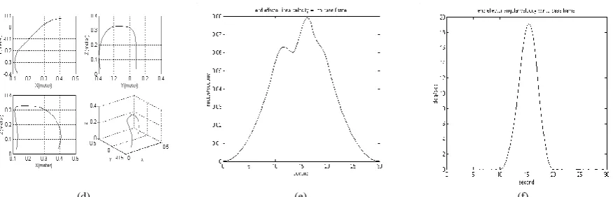
From figure 5 it can be seen that joint-02 and 03 are subjected to the maximum movement. These are the shoulder and elbow joints respectively. Thus, it can be understood that these joints play a major role in manipulating an object in the space by ER-V plus robotic system. Joint–04 and 05 are subjected to the minimum movement. Movement for joint-05 is zero.
(d) (e) (f)
Fig. 5 position, velocity and acceleration (a) joint angle variation along the trajectory (b) joint velocity variation along the trajectory (c) End-effector‟s Cartesian path derived (d) End-effector‟s linear velocity along trajectory (e) End-effector‟s angular velocity along trajectory
V. CONCLUSIONS
This paper presents a general method of carrying out differential motion analysis of a robot manipulator of industrial type, considering its geometric and kinematic parameters. The joint trajectories have been modeled using 5-cubic type of trajectory planning scheme whose coefficients have been determined by using MATLAB codes. Proper trajectory between given initial and final point of the robot hand motion is of considerable importance. The trajectory should give a smooth motion of joints and hence robot hand. Moreover, minimum jerk trajectory is desirable for its similarity to human joints movements and to limit excessive wear on the robot and the excitation of resonance so that the robot life span is long.
REFERENCES
[1] Daniel Martins, Raul Guenther, “Hierarchical kinematic analysis of robots”, Mechanism and Machine Theory 38, 2003, pp 497-518.
[2] Eva Dyllong and Antonio Visioli, “Planning and real-time modifications of a trajectory using spline techniques”, Robotica, volume 21, 2003, pp.475-482.
[3] L.E.Gonchar, D.Engel, J.Raczkowsky, and H.Worn, “Simulation for path planning and motion control for medical robot”, Proceedings of the workshop on Computer Science and Information Technologies CSIT‟2000, Ufa, Russia, 2000.
[4] John J.Craig, ”Introduction to Robotics: Mechanics and Control”, second edition, Addision wesley, 1989.
[5] K.S.Fu, R.C.Gonzalez, C.S.G.Lee, “ROBOTICS: Control, Sensing, Vision and Intelligence”, McGraw-Hill international edition, 1987. [6] Richard P. Paul, “ROBOT MANIPULATORS: Mathematics Programming and Control”, MIT Press, Cambridge, MA, 1981. [7] R.K.Mittal, I.J.Nagrath, “Robotics and Control”, Tata McGraw Hill Publishing Company Limited, 2003.
[8] SCORBOT-ER Vplus User‟s Manual, 3rd edition, ESHED ROBOTEC.