Volume 9, No. 3, May-June 2018
International Journal of Advanced Research in Computer Science
RESEARCH PAPER
Available Online at www.ijarcs.info
ISSN No. 0976-5697
THE TASK ALLOCATION MODEL IN COMMUNICATION
CHANNEL DELAY
Kamini Raikwar
Research Scholar Department of Mathematics M.G.C.G.V. Chitrakoot (M.P.), India
Virendra Upadhyay Department of Mathematics
M.G.C.G.V. Chitrakoot (M.P.), India Manoj Kumar Shukla
Department ofMathematics, InstituteforExcellenceinHigherEducation,
Bhopal, (M.P.) India
Abstract : In this paper a heuristics approach for task allocation in a distributed computing system has been discussed. This performs static allocation and provide near optimal results. The suggested algorithm is coded in Mat Lab and implemented on a Dual Core machine and found the performance of the developed algorithm is satisfactory.
Keywords: Distributed Computing System, mainframes, computational
1. INTRODUCTION
A Distributed Computing System (DCS) consists of any number of possible configurations, such as mainframes, personal computers, workstations, minicomputers, and so on. The goal of distributed computing is to the transparent data distribution within a local network. A user-oriented definition of distributed computing is"Multiple Computers, utilized cooperatively to solve problems" has been reported by {Sita [04], Chia [03], and Bhut [02]}. Distributed computing systems are of current interest for the researchersdue to the advancement of microprocessor technology and computer networks {Till [05], Aror [01]}. In a DCS, the execution of a program may be distributed among several processing elements to reduce the overall cost of execution by taking advantage of inhomogeneous computational capabilities and other resources within the system. The task allocation in a DCS finds extensive applications in the faculties, where large amount of data is to be processed in relatively short period of time, or where real-time computations are required such as, Meteorology, Cryptography, Image Analysis, Signal Processing, Solar and Radar Surveillance, Simulation of VLSI circuits and Industrial process monitoring are areas of such applications.
2. PROBLEM STATEMENT
Consider a DCS consisting a set of n processors
𝑃 = {𝑝1, 𝑝2, … . 𝑝𝑛}, interconnected by
communication links and a set of m tasks 𝑇 =
{{𝑡1, 𝑡2, … . 𝑡𝑚} where 𝑚 > 𝑛. An allocation of tasks to
Processors is defined by a function Aalloc from
the set 𝑇 of tasks to the set 𝑃 of processors such
that:
Aalloc: 𝑇 → 𝑃 ,where Aalloc (𝑖) = 𝑗 if task 𝑡𝑖 is
assigned to processor 𝑝𝑗 , 1 ≤ 𝐼 ≤ 𝑚, 1 ≤
𝑗 ≤ 𝑛.
While designing the model it is assumed that Execution Cost (EC) of each task on all the Processors and the Data Transfer Rate (DTR) between the tasks is known and will be taken in the form Execution Cost Matrix [ECM (,)] of order m x n, and Data Transfer Rate Matrix [DTRM(,)] of order m respectively. The communication channel delay is also considered and taken in the form of Channel Delay Matrix
[CDM (,)] of order 𝑚.
3. PROPOSED METHOD
The allocation of tasks is to be carried out so that each task is assigned to a processor whose capabilities are most appropriate for the tasks, and their processing cost is to be minimized. The present model passes through the following phases.
Phase –I
Average Load:
The average load Lavg and Total Load (TL) is to be assigned on processor pj with 05% Tolerance Factor (TF) has to be calculated as:
𝐿𝑎𝑣𝑔(𝑝𝑗) = 𝑒𝑐𝑖𝑗
𝑚 1 < 𝑖 < 𝑚,1 < 𝑗 < 𝑛 … … … 3.1
𝐿𝑇 = ∑ 𝐿𝑎𝑣𝑔(𝑝𝑗) + 𝑇𝐹 … … … 3.2
𝑤ℎ𝑒𝑟𝑒 𝑇𝐹 = (𝐿𝑎𝑣𝑔(𝑝𝑗)) ∗ 0.5
100 𝑎𝑛𝑑 𝑗 =
Selection of “𝒏” Task on the basis of minimum DTR:
The upper diagonal values of the DTRM (,) are stored in Maximum Data Transferred Rate Matrix
MAXDTRM (,) of order 𝑚(𝑚 − 1)/2 by 3 the
first column represents first task (say rth task), second column represent the second task (say sth task) and third column represent the DTR (drs) between these rth and sth tasks. The MAXDTRM (,) is then stored in ascending order
assuming the third column as sorted key and select first tasks “n” which and store the tasks in
𝑇𝑡𝑎𝑠𝑘𝑠 (𝑗) (where 𝑗 = 1,2, … , 𝑛) and also store
the remaining 𝑚 − 𝑛 tasks in another linear array
𝑇𝑁𝑡𝑎𝑠𝑘𝑠(𝑘) (where 𝑘 = 1,2, … , 𝑚 − 𝑛).
Assignment: To get the initial assignment store the ECM (,) in NECM (,) NECM (,) ← ECM (,)
then reduce the NECM(i,j) ( 𝑤ℎ𝑒𝑟𝑒 𝑖 =
1,2, … 𝑛 𝑎𝑛𝑑 𝑗 = 1,2, … 𝑛) in the square matrix
of order n by deleting tasks stored in TNtasks (k) which is the intersection of Ttasks(i) and apply the YAS-Algorithm developed by Yadav et al [04].
The initial allocation is stored in an array 𝑇𝑎𝑠𝑠(𝑗)
(where j = 1,2,…,n) and also the processor position are stored in a another linear array Aalloc (j). Get the value of TTASK (j) by adding the
values of Aalloc (𝑗) if a task is assigned to a
processor otherwise continue. Select a task from TNtasks (k) (where k = 1,2,….…m-n) for assignment say tk and assign task to processor pj where the value of EC in minimum. Store the assignment and their position in Tass(j) and Aalloc (j) respectively and modify the TTASK (j) by adding the value of Aalloc (j). The TNtasks (k) is also modify the by deleting the tasks tk. This process of assignment is continuing till the remaining “m-n” tasks are get allocated.
Phase -II
After completing the allocations the Processor’s
Wise Execution Cost (PEC) ecij (1 ≤ 𝑖 ≤
𝑚 , 1 ≤ 𝑗 ≤ 𝑛) of each task ti on the processor
pj is calculated using the following equation
𝑃𝐸𝐶(𝐴𝑎𝑙𝑙𝑜𝑐)𝑗= ∑1≤𝑖≤𝑚𝑒𝑐𝑖,
𝑖∈𝑇𝑆𝑗
𝐴𝑎𝑙𝑙𝑜𝑐(𝑗) … … … 3.3
𝑤ℎ𝑒𝑟𝑒 𝑇𝑆𝑗 = {𝑖:𝐴𝑎𝑙𝑙𝑜𝑐(𝑖) = 𝑗, 𝑗 = 1,2, … … … 𝑛
Inter Processor Communication (IPC):
The Inter Processor Communication cost of the interacting tasks ti and tk is depends upon the per unit data transfer rate dik during the program execution is determined by using the equation given below Inter Processor Communication with delay (IPCWD) is calculated by the equation given below
𝐼𝑃𝐶𝑊𝐷(𝐴𝑎𝑙𝑙𝑜𝑐)𝑗 = [min(𝑒𝑐𝑖𝑗∗ 𝑑𝑖𝑗)] ∗ 𝑐𝑑𝑖𝑗,
𝑗 = 1,2, … . . 𝑛 𝑎𝑛𝑑 𝑖 = .1,2 … . 𝑚 … … … 3.4
Where 𝑐𝑑𝑖𝑗 s the delay channel.
Inter Processor Communication without delay (IPCWOD) is calculated by the equation
Given below
𝐼𝑃𝐶𝑊𝑂𝐷 (𝐴𝑎𝑙𝑙𝑜𝑐)𝑗 =[min(𝑒𝑐𝑖𝑗 ∗ 𝑑𝑖𝑗)] 𝑗 =
1,2, … . . 𝑛 𝑎𝑛𝑑 𝑖 = .1,2 … . 𝑚 … … . .3.4.1 Calculate the Overall Processors Cost [OPC] with
delay and without delay calculated as
𝑂𝑃𝐶𝑊𝐷(𝐴𝑎𝑙𝑙𝑜𝑐)𝑗 = 𝑃𝐸𝐶(𝐴𝑎𝑙𝑙𝑜𝑐)𝑗+
𝐼𝑃𝐶𝑊𝐷(𝐴𝑎𝑙𝑙𝑜𝑐)𝑗 … … … … 3.5
𝑂𝑃𝐶𝑊𝐷(𝐴𝑎𝑙𝑙𝑜𝑐)𝑗 = 𝑃𝐸𝐶(𝐴𝑎𝑙𝑙𝑜𝑐)𝑗
+ 𝐼𝑃𝐶𝑊𝑂𝐷(𝐴𝑎𝑙𝑙𝑜𝑐)𝑗… … … … 3.5.1
and find the average Overall Processors Cost [OPC]
The Mean Service Rate [MSR] with delay and without delay of the processors are calculated by using the equation described below and store the
results in MSR (𝐴𝑎𝑙𝑙𝑜𝑐)𝑗
( 𝑤ℎ𝑒𝑟𝑒 𝑗 = 1,2, … , 𝑛).
𝑀𝑆𝑅𝑊𝐷(𝐴𝑎𝑙𝑙𝑜𝑐)𝑗= 1
𝑂𝑃𝐶𝑊𝐷(𝐴𝑎𝑙𝑙𝑜𝑐)𝑗 𝑊ℎ𝑒𝑟𝑒 𝑗 =
1,2, … 𝑛… … … . . 3.6
𝑀𝑆𝑅𝑊𝐷(𝐴𝑎𝑙𝑙𝑜𝑐)𝑗=
1
𝑂𝑃𝐶𝑊𝐷(𝐴𝑎𝑙𝑙𝑜𝑐)𝑗 𝑊ℎ𝑒𝑟𝑒 𝑗 =
1,2, … 𝑛… … … . . 3.6.1
The throughputs of the processors with delay and without delay are calculated by using the equation given below and store the results in a linear arrays 𝑇𝑅𝑃 (𝐴𝑎𝑙𝑙𝑜𝑐)𝑗 , where 𝑗 = 1,2 … … . , 𝑛.
𝑇𝑅𝑃(𝐴𝑎𝑙𝑙𝑜𝑐)𝑗 = 𝑇𝑇𝐴𝑆𝐾(𝐴𝑎𝑙𝑙𝑜𝑐)𝑗
𝑂𝑃𝐶𝑊𝐷(𝐴𝑎𝑙𝑙𝑜𝑐)𝑗 𝑤ℎ𝑒𝑟𝑒 𝑗 =
1,2, … … … 𝑛 … … … 3.7
𝑇𝑅𝑃(𝐴𝑎𝑙𝑙𝑜𝑐)𝑗 = 𝑇𝑇𝐴𝑆𝐾(𝐴𝑎𝑙𝑙𝑜𝑐)𝑗
𝑂𝑃𝐶𝑊𝐷(𝐴𝑎𝑙𝑙𝑜𝑐)𝑗 𝑤ℎ𝑒𝑟𝑒 𝑗 =
Finally, Critical Transmission Delay [CTD] and the Optimal Processing Cost (OPC) with delay and without delay have been determined. The
maximum value of 𝑂𝑃𝐶 (𝐴𝑎𝑙𝑙𝑜𝑐)𝑗will be the Total
System Cost (TSC) which shell be the optimal cost of the DCS.
3.4 ALGORITHM:
Step1: Input; m, n, ECM (,), DTRM (,) and CDM (,)
Step2: 𝑓𝑜𝑟 𝑖 ← 1 𝑡𝑜 𝑚 𝑑𝑜 𝑓𝑜𝑟 𝑗 ← 1 𝑡𝑜 𝑛 𝑑𝑜
Determine the Total Load (TL) to be assigned on processor pj with 05% Tolerance
Factor (TF) by using the equation (1) and (2) respectively.
𝑟𝑒𝑝𝑒𝑎𝑡
𝑟𝑒𝑝𝑒𝑎t
Step3: 𝑘 ← 𝑚(𝑚 − 1)/2
𝑡 ← 𝑚 − 𝑛
𝑓𝑜𝑟 𝑖 ← 1 𝑡𝑜 𝑚 𝑑𝑜 𝑓𝑜𝑟 𝑗 ← 1 𝑡𝑜 𝑘 𝑑𝑜
Store the “𝑘” upper diagonal value of DTRM (,) in
MAXDTRM (,)
MAXDTRM (,) ← DTRM (,)
Arrange the MAXDTRM (,) ascending order 𝑟𝑒𝑝𝑒𝑎𝑡
𝑟𝑒𝑝𝑒𝑎𝑡
Step4: 𝑓𝑜𝑟 𝑖 ← 1 𝑡𝑜 𝑛 𝑑𝑜 𝑓𝑜𝑟 𝑗 ← 1 𝑡𝑜 𝑛 𝑑𝑜
Store the ECM (,) in NECM (,) NECM (,) ← ECM (,)
𝑟𝑒𝑝𝑒𝑎𝑡 𝑟𝑒𝑝𝑒𝑎𝑡
Step5: 𝑐𝑜𝑢𝑛𝑡 ← 𝑛 𝑓𝑜𝑟 𝑖 ← 1 𝑡𝑜 𝑚 𝑑𝑜 𝑓𝑜𝑟 𝑗 ← 1 𝑡𝑜 𝑘 𝑑𝑜
Pick-up the minimum value from MAXDTRM (,) say 𝑡𝑗 , 𝑡𝑘
𝐼𝑓 𝑛 = 𝑐𝑜𝑢𝑛𝑡; Then
store the tasks in a linear array Ttasks( ) and go to the step-5
else;
Repeat 𝑓𝑜𝑟 𝑖
if MAXDTRM(i,j)< MAXDTRM(i,k) 𝑏𝑚𝑖𝑛 ← 𝑀𝐴𝑋𝐷𝑇𝑅𝑀(𝑖, 𝑗) 𝑢𝑛𝑡𝑖𝑙 𝑗 = 𝑘
𝑏𝑚𝑖𝑛 < 𝑀𝐴𝑋𝐷𝑇𝑅𝑀(𝑖, 𝑘) 𝑢𝑛𝑡𝑖𝑙 𝑗 = 𝑘 𝑒𝑛𝑑 𝑖𝑓
check the corresponding position of bmin MAXDTRM(,) (say tl) and give one increment to count
𝑐𝑜𝑢𝑛𝑡 ← 𝑐𝑜𝑢𝑛𝑡 + 1
store the tasks in a linear array Ttasks( ) also store the remaining m-n tasks in TNtasks( )
𝑟𝑒𝑝𝑒𝑎𝑡
𝑟𝑒𝑝𝑒𝑎𝑡
Step 6: Reduce MAXDTRM (,) and also modify the NECM (,) by eliminating the tasks stored in Ttasks( )
Step-7: Apply the YAS-Algorithm to get the initial allocation and store the assignment in an linear array
Tass(j) (𝑤ℎ𝑒𝑟𝑒 𝑗 = 1,2, … , 𝑛) also the processor
position are stored in a another linear array Aalloc(j). Get the
value of TTASK (j) by adding the values of
𝐴𝑎𝑙𝑙𝑜𝑐 (𝑗) if a task
is assigned to a processor otherwise continue.
Step-7.1:
𝑓𝑜𝑟 𝑖 ← 1 𝑡𝑜 𝑚 𝑑𝑜
𝑠𝑡𝑜𝑟𝑒 𝑡ℎ𝑒 𝑇𝑁𝑡𝑎𝑠𝑘𝑠( ) 𝑖𝑛 𝑇𝑛𝑜𝑛 − 𝑎𝑠𝑠( ) 𝑇𝑛𝑜𝑛 − 𝑎𝑠𝑠( ) ← 𝑇𝑁𝑡𝑎𝑠𝑘𝑠( )
𝑟𝑒𝑝𝑒𝑎𝑡 Step:7.2:
𝑓𝑜𝑟 𝑖 ← 1 𝑡𝑜 𝑚 − 𝑛 𝑑𝑜 𝑓𝑜𝑟 𝑗 ← 1 𝑡𝑜 𝑛
Select a task from TNtasks (k) (𝑤ℎ𝑒𝑟𝑒 𝑘 =
1,2, … , 𝑚 − 𝑛) for assignment say 𝑡𝑖 and
assign task to processor pj where the value of ecij
is minimum.
𝐴𝑎𝑙𝑙𝑜𝑐(𝑘) ← 𝑗;
𝑛𝑜𝑚𝑎𝑑𝑒 ← 𝑛𝑜𝑚𝑎𝑑𝑒 + 1;
𝑇𝑎𝑠𝑠 ← 𝑇𝑎𝑠𝑠 ∪ {𝑡𝑘};
𝑟𝑒𝑝𝑒𝑎𝑡
𝑟𝑒𝑝𝑒𝑎𝑡
This process is continuing till the remaining “𝑚 −
𝑛” tasks are get allocated.
𝑓𝑜𝑟 𝑘 ← 1 𝑡𝑜 𝑚 𝑑𝑜 𝑓𝑜𝑟 𝑗 ← 1 𝑡𝑜 𝑛 𝑑𝑜
Compute the final 𝑃𝐸𝐶 (𝐴𝑎𝑙𝑙𝑜𝑐)𝑗 using the
equation (3.3) 𝑟𝑒𝑝𝑒𝑎𝑡
𝑟𝑒𝑝𝑒𝑎𝑡
Step-9:
𝑓𝑜𝑟 𝑘 ← 1 𝑡𝑜 𝑚 𝑑𝑜 𝑓𝑜𝑟 𝑗 ← 1 𝑡𝑜 𝑛 𝑑𝑜
Compute the Inter Processor Communication Cost
IPC (𝐴𝑎𝑙𝑙𝑜𝑐) 𝑗 of the interacting tasks ti and tk by
using the equation (3.4) and (3.4.1) 𝑟𝑒𝑝𝑒𝑎𝑡
𝑟𝑒𝑝𝑒𝑎𝑡 Step-10:
𝑓𝑜𝑟 𝑖 ← 1 𝑡𝑜 𝑚 𝑑𝑜
Determine the finally, Overall Processors Cost
OPC (𝐴𝑎𝑙𝑙𝑜𝑐)𝑗 by using the equation (3.5) and
(3.5.1) 𝑟𝑒𝑝𝑒𝑎𝑡 Step-11:
𝑓𝑜𝑟 𝑖 ← 1 𝑡𝑜 𝑛 𝑑𝑜
Compute the mean service rate MSR (𝐴𝑎𝑙𝑙𝑜𝑐)𝑗
by using the equation (3.6) and (3.6.1) 𝑟𝑒𝑝𝑒𝑎𝑡
Step-12:
𝑓𝑜𝑟 𝑖 ← 1 𝑡𝑜 𝑛 𝑑𝑜
Compute the processor’s throughput by using the equation (3.7) and (3.7.1)
𝑅𝑒𝑝𝑒𝑎𝑡
Step-13: Calculate the total Critical Transmission Delay [CTD] and the maximum value of
𝑂𝑃𝐶 (𝐴𝑎𝑙𝑙𝑜𝑐)𝑗 i.e .the Total System Cost
Step-14: 𝑆𝑡𝑜𝑝.
3.5 IMPLEMENTATION OF THE ALGORITHM:
Example:
To justify the application and usefulness of the present algorithm an example of a DCS is
Considered which is consisting 𝑜𝑓 𝑛 = 3 the set
of processors 𝑃 = {𝑝1, 𝑝2, 𝑝3} connected by
anarbitrary network and m = 6 the set of tasks T=
{𝑡1, 𝑡2, 𝑡3, 𝑡4, 𝑡5, 𝑡6} which may be portion of
an executable code or a data file.
Step1:
Input of the Algorithm: Data required by the algorithm is given below:
Number of processors available in the system (n) = 3
Step2:After Implementation of the Algorithm’s steps the Average load to be assigned on the processors has been given in table 3.1
Table 3.1
Processors Average execution cost
P1 5
P2 3
P3 4
Total Load 12
05% Tolerance Factor [TF] 0.6 ( = 0.5 say)
Total Average load on the processor= Total load + TF] 12+0.5= 12.5
Step3:
The MAXDTRM (,) is stored in ascending order assuming the third column as sorted key and
select those tasks “𝑛 = 3” which has minimum
DTR and store the tasks in Ttasks(j) (𝑤ℎ𝑒𝑟𝑒 𝑗 =
1,2, … , 𝑛) and also store the remaining m-n tasks
1,2, … , 𝑚 − 𝑛).
t1 t8 0.000
t2 t3 0.000
t2 t4 0.000
t2 t5 0.000
t2 t6 0.000
t2 t7 0.000
t3 t7 0.000
t3 t8 0.000
t5 t6 0.000
t5 t7 0.000
t5 t8 0.000
t1 t6 0.125
MAXDTRM (,) = t6 t8 0.125
t1 t5 0.167
t6 t7 0.176
t2 t8 0.200
t4 t5 0.200
t4 t8 0.200
t7 t8 0.200
t1 t3 0.250
t3 t4 0.250
t1 t2 0.333
t3 t5 0.333
t4 t6 0.333 t1 t4 0.500 t3 t6 0.500 t4 t7 0.500 t1 t7 1.000
Step4: Store the ECM (,) in NECM,) as: p1 p2 p3 p1 p2 p3 t1 6 3 5 t1 6 3 5 t2 4 2 3 t2 4 2 3 t3 3 1 2 t3 3 1 2 NECM(,) = t4 5 2 ∞ ← ECM(,) = t4 5 2 ∞ t5 3 4 2 t5 3 4 2 t6 6 ∞ 6 t6 6 ∞ 6 t7 5 6 7 t7 5 6 7
Step5:
Ttasks( ) = { t1 t8 t5} TNtasks( ) ={ t2 t3 t4 t6 t7 }
Step6:
Reduced NECM(,) and MXDTRM(,) p1 p2 p3
t1 6 3 5 NECM(,) = t5 3 4 2
t8 ∞ 2 5 t2 t3 0.000 t2 t4 0.000 t2 t5 0.000 t2 t6 0.000 t2 t7 0.000 t3 t7 0.000 t3 t8 0.000 t5 t6 0.000 t5 t7 0.000 t1 t6 0.125 MAXDTRM (,) = t6 t8 0.125 t1 t5 0.167 t6 t7 0.176 t2 t8 0.200 t4 t5 0.200 t4 t8 0.200 t7 t8 0.200 t1 t3 0.250 t3 t4 0.250 t1 t2 0.333 t3 t5 0.333 t4 t6 0.333 t1 t4 0.500 t3 t6 0.500 t4 t7 0.500 t1 t7 1.000
Step7:
Initial assignments are obtained by applying the YAS-Algorithm developed by Yadav et
al [Yada04 ] are given in Table 3.2:
Table 3.2 Initial
Assignment
Tasks Processor EC
t5 p1 3
t8 p3 5
t1 p2 3
Step7.1:
𝑇𝑛𝑜𝑛 − 𝑎𝑠𝑠 () ← 𝑇𝑁𝑡𝑎𝑠𝑘𝑠( ) 𝑇𝑛𝑜𝑛 − 𝑎𝑠𝑠 () = { 𝑡2 𝑡3 𝑡4 𝑡6 𝑡7 } 𝐴𝑎𝑙𝑙𝑜𝑐 (𝑗) = {1, 3, 2} 𝑎𝑛𝑑 𝑇𝑇𝐴𝑆𝐾 (𝑗) = { 1,1,1}
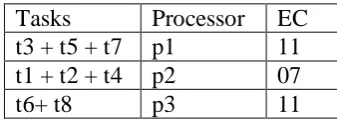
[image:8.595.387.556.598.659.2]After Implementing the Step-7.2 the following final assignment are obtained.
Table 3.3: Final Assignment
Tasks Processor EC
t3 + t5 + t7 p1 11
t1 + t2 + t4 p2 07
t6+ t8 p3 11
The final 𝐴𝑎𝑙𝑙𝑜𝑐(𝑗) = {1,3,2,1,1,2,2,3,3} and
𝑇𝑇𝐴𝑆𝐾 (𝑗) = { 3,3,2}, Table 3.3 shows the
final assignment after Implementation of
assignment procedure described in section 3.3 in the
Table – 3.4: Processors EC IPC
without Delay
IPC with Delay
OPC without Delay
OPC with Delay
MSR without Delay
MSR with Delay
TRP without Delay
TRP with Delay
Total critical Transmission Delay
1 2 3 4 5=2+3 6= 2+4 7 8 9 10 11=6-5
P1 11.000 5.079 7.658 16.079 18.658 0.062 0.054 0.124 0.107 2.579 P2 7.000 4.882 7.364 10.882 13.364 0.092 0.075 0.276 0.224 2.482 P3 11.000 3.705 6.510 13.705 16.510 0.073 0.061 0.219 0.182 2.805
REFERENCES
[1] Arora, R.K., and Rana, S.P., “On module assignment in two processors distributed Systems”,Information Processing Letters, Vol. 9, No. 3, pp. 113-117, 1979. [2] Bhutani, K.K., “Distributed Computing”, The Indian
Journal ofTelecommu nication, pp. 41- 44, 1994. [3] Chiao – Pin Bao, Ming-Chi Tsai, Meei-Ing Tsai., 2007,
“A new Approach to Study the Multi Objective
Assignment Problem”, WHAMPOA- An Interdisciplinary journal, 53 (2007), PP. 123- 132. [4] Sitaram, B. R., “Distributed computing – a user’s view
point”, CSI Communications, Vol. 18, No. 10, pp.26-28, 1995.