Discrete Maximum Principle and Energy Stability of Compact Difference Scheme for the Allen-Cahn Equation

Discrete Maximum Principle and Energy Stability of Compact

Difference Scheme for the Allen-Cahn Equation

Dan Tian1 , Yuanfeng Jin1† and Gang Lu2

1 Department of Mathematics, Yanbian University, Yanji 133001, P.R. China; 2 Department of Mathematics, School of Science, ShenYang University of Technology, Shenyang 110870, P.R. China (email:

[email protected], [email protected], [email protected])

Abstract

In the paper, a fully discrete compact difference scheme with O(τ2_+h4_{) precision is established}

by considering the numerical approximation of the one-dimensional Allen-Cahn equation. The numerical solutions satisfy discrete maximum principle under reasonable step ratio and time step constraint is proved. And the energy stability for the fully discrete scheme is investigated. An example is finally presented to show the effectiveness of scheme.

Key words: Allen-Cahn Equation; Compact Difference Scheme; Maximum Principle; Energy

Stability.

1

Introduction

The phase field model is a mathematical model which is described by partial differential equations. Due to its complexity, the numerical simulation of phase field are all along the very important problem which has been discussed at home and abroad, there are some theory and realistic sense for us to deal with the problems. In 1979, Allen and Cahn introduced the Allen-Cahn equation to describe the anti-phase boundary motion in the crystal. This equation describes fluid dynamics problems and reaction diffusion problems in materials science, and also proposes the same model in the study of many diffusion phenomena such as competition and rejection of biological populations, migration processes of riverbeds. For describing the anti-phase boundary motion in a crystal, since there is no exact solution for such a phase field model, the model was simulated by numerical method. At present numerical approximation methods for such phase field models include finite difference methods, finite element methods [8, 9], and spectral methods [6].

This paper presents the compact difference method to approximate the one-dimensional nonlinear Allen-Cahn equation with initial boundary conditions.

   

  

∂u ∂t =ε

2_{∆u−f(u), x∈Ω, t∈[0, T].}

u(x,0) =u0(x), x∈Ω¯.

u|_∂Ω = 0, t∈[0, T].

(1.1)

where u indicates the concentration of a metal part in a binary alloy, the parameter ε >0 is the width of the interface, and the nonlinear term f(u) =u3−u.

Define the energy function in L2- space

E(u) = I

Ω

(F(u)−1 2ε

2_{u4u)dx. (1.2)}

1

where F(u) = 1₄(u2−1)2. One of the intrinsic properties of the Allen-Cahn equation is that the energy function is decreasing with time,

d

dtE(u)≤0, ∀t >0. (1.3)

It is known that the Allen-Cahn equation satisfies the maximum principle and energy stability. Then is it true that these properties are true for numerical approximation solutions? In 2010, Shen Jie established first-order semi-implicit scheme, order semi-implicit scheme and second-order implicit scheme for Allen-Cahn equation and Cahn-Hilliard equation, and completed energy digressive stability analysis and error analysis [10]. In 2016, Zhang Jiaqi and Hou Tianliang considered three discrete schemes of the Allen-Cahn equation: stable first-order linear implicit-explicit scheme, stable second-order nonlinear correction Crank-Nicolson scheme and stable second-order linear Leap-Frog scheme, proved that these three schemes satisfy the discrete maximum principle and energy stability [1]; Tang Tao proved the maximum principle and the unconditional stability of the first-order implicit-explicit scheme of the Allen-Cahn equation, and gave an error analysis [2]. In 2017, Zheng Nan gave two high-efficiency numerical schemes for solving the Allen-Cahn equation, compared the operational efficiencies of the two numerical solutions, and verified the energy diminishing law by numerical examples [3]; Hou Tian Liang and Tang Tao established the second-order Crank-Nicolson scheme in time and second-order central difference approximation in space for fractional-in-space Allen-Cahn equation, which proved that the numerical solution satisfies the discrete maximum principle and energy stability under reasonable time step constraints, and gave an error analysis [5]. Based on the existing finite difference methods, a discrete format with four-order precision–the compact difference scheme, is established to perform related numerical analysis. The main research is two aspects: one is the discrete maximum principle: the numerical solutions for (1.1) can be bounded by 1 under the condition that the initial data is bounded by 1; the other is the energy stability: the defined discrete energy is decremented.

2

Establishment of the Compact Difference Scheme

In this section, the compact difference scheme with O(τ2 +h4) precision is established for the one-dimensional Allen-Cahn equation (1.1) .

First, three common numerical differential formulas were described. Let h >0 and c be two constants,

(1)If g(x)∈C2[c−h, c+h], there is

g(c) = 1

2[g(c−h) +g(c+h)]−

h2

2 g

00

(ξ1), c−h < ξ1< c+h. (2.1)

(2)If g(x)∈C3[c−h, c+h], there is

g0(c) = 1

2h[g(c+h)−g(c−h)]− h2

6 g

000

(ξ2), c−h < ξ2 < c+h. (2.2)

(3)If g(x)∈C6[c−h, c+h], there is 1

12[g

00

(c−h) + 10g00(c) +g00(c+h)] = 1

h2[g(c+h)−2g(c) +g(c−h)] +

h4

240g

(6)_(ξ 3),

Next, we divide equally the solution interval x ∈ Ω, t ∈ [0, T] into N equal segments. Let

h = _NΩ, τ = _NT, where h and τ are the space step and time step. Denote Ωhτ = {uni|0 ≤ i ≤

N,0≤n≤N} is called grid function, introduce the following notations,

δtu n+1₂

i =

1

τ(u

n+1

i −uni). δ2xuni = 1

h2(u

n

i+1−2uni +uni−1).

un+

1 2

i =

1 2(u

n+1

i +uni). (u n+1₂

i )3 = 1 2[(u

n+1

i )3+ (uni)3]. where

un_i =u(xi, tn), 0≤i≤N, 0≤n≤N.

Let u={ui|0≤i≤N}, define the operator

(Au)i=  

 1

12(ui−1+ 10ui+ui+1), 1≤i≤N −1,

ui, i= 0, N.

(2.4)

Considering equation (1.1) at the point (xi, tn+1₂), we obtain

∂u

∂t(xi, tn+12) =ε 2∂2u

∂x2(xi, tn+₂1)−f(xi, tn+1₂), 0≤i≤N, 0≤n≤N−1. (2.5)

Using formula (2.1) and (2.2), we have

∂u

∂t(xi, tn+12) = 1

τ[u(xi, tn+1)−u(xi, tn)]− τ2

24·

∂3u

∂t3(xi, θin).

∂2u

∂x2(xi, tn+1₂) =

1 2[

∂2u

∂x2(xi, tn) +

∂2u

∂x2(xi, tn+1)]−

τ2

8 ·

∂4u

∂x2_∂t2(xi,θein).

where θin,eθ_in(t_n, t_n+1). Then we get

δtu n+1₂

i =ε

2_·1

2[

∂2u

∂x2(xi, tn) +

∂2u

∂x2(xi, tn+1)]−f(xi, tn+1₂)

+ [ 1 24·

∂3u

∂t3(xi, θin)−

ε2

8 ·

∂2v

∂t2(xi,θein)]τ

2_{, 0≤i≤N, 0≤n≤N −1. (2.6)}

Acting operator Aon both sides of the above formula, we obtain

Aδtu n+1₂

i =ε2· 1 2[A

∂2_u

∂x2(xi, tn) +A

∂2_u

∂x2(xi, tn+1)]− Af(xi, tn+1₂)

+A[ 1 24·

∂3u

∂t3(xi, θin)−

ε2

8 ·

∂2v

∂t2(xi,θein)]τ

2_{, 1≤i≤N−1, 0≤n≤N −1. (2.7)}

Using formula (2.3), we have

A∂ 2_u

∂x2(xi, tn) =δ 2

xuni +

h4

240·

∂6u

∂x6(ξin, tn).

where ξin(xi−1, xi+1). Add the two equations of (2.7) that labeled n and n+ 1, and divide by 2,

we have

1 2[A

∂2u

∂x2(xi, tn) +A

∂2u

∂x2(xi, tn+1)] =

1 2(δ

2

xuni +δx2uni+1) +

h4

240·

∂6u

where ξ_in(xi−1, xi+1)tin(tn, tn+1).

Substituting (2.8) into (2.7), we obtain

Aδtu n+1

2

i =ε

2(δ2xuni +δ2xuni+1)

2 − Af(xi, tn+12) +Rin, 1

≤i≤N−1, 0≤n≤N−1. (2.9)

where

Rin=A[ 1 24 ·

∂3u

∂t3(xi, θin)−

ε2

8 ·

∂2v

∂t2(xi,θein)]τ 2₊ ε2

240·

∂6u

∂x6(ξin, tin)h4. (2.10) In (2.9) , omit the error term Rin and substitute the following

f(xi, tn+1₂) =

(un_i+1)3+ (un_i)3

2 −

un_i+1+un_i

2 .

Then we can get the Allen-Cahn equation (1.1) corresponding compact difference scheme:

Au n+1

i −uni

τ +A[

(un_i+1)3+ (un_i)3

2 −

un_i+1+un_i

2 ] =

ε2

2(δ

2

xuni+1+δx2uni), (2.11) 1≤i≤N−1, 0≤n≤N−1.

Finally, we use the second-order central finite difference to approximate the spatial derivatives and denote Dh as the corresponding discrete matrix, so Dh is given by

Dh = 1

h2



    

−2 1 0 0

1 −2 . .. 0

0 . .. ... 1

0 0 1 −2



    

N×N

. (2.12)

where N indicates the number of internal nodes in the space, and h indicates the space step. It can be verified that the discrete matrix Dh satisfies the following properties:

(1) Dh is symmetric;

(2) Dh is negative semidefinite, i.e.

UTDhU ≤0, ∀ U ∈RN; (2.13)

(3)Elements of Dh satisfy

dii=−b <0, b≥ max

1≤i≤N X

j6=i

|bij|. (2.14)

To represent the average operator, A can be expressed as:

A= 

    

10 12

1

12 0 0 1

12 10

12 . .. 0

0 . .. ... ₁₂1 0 0 ₁₂1 10₁₂



    

N×N

. (2.15)

(2) A is positive, i.e.

UTAU >0, ∀U ∈RN; (2.16)

(3)Elements of A satisfy

aij >0, kAk∞= max 1≤i≤N

N X

j=1

aij = 1. (2.17)

Substituting the matrix Dh and A into (2.11), we construct the compact difference scheme as follow:

AU

n+1_−Un

τ +A[

(Un+1).3−Un+1

2 +

(Un).3−Un

2 ] =

ε2(DhUn+1+DhUn)

2 . (2.18)

where

Un:= (U₁n, U₂n,· · ·, U_Nn)T,

(Un).3:= ((U₁n)3,(U₂n)3,· · ·,(U_Nn)3)T.

On both sides of the compact difference scheme (2.18) multiplied by matrix A−1, we obtain,

Un+1−Un τ + [

(Un+1).3−Un+1

2 +

(Un).3−Un

2 ] =

ε2

2A

−1_D

h(Un+1+Un). (2.19) It can be verified that the matrix A−1Dh satisfies the following properties:

(1) A−1Dh is symmetric; (2) A−1Dh is negative, i.e.

UTA−1DhU ≤0, ∀ U ∈RN. (2.20)

3

The Discrete Maximum Principle

Theorem 3.1. Let us consider the Allen-Cahn problem (1.1). If the initial value is bounded by 1,

i.e. max xΩ

|u0(x)| ≤1, then the numerical solution of the fully discrete scheme (2.18) is also bounded by 1 in the sense that kUnk∞ ≤1 for all n≥ 1, and the step ratio satisfies 1₆ ≤λ≤ 5₆, and the time step size satisfies 0< τ ≤min{λ−1₆,1−6₅λ}.

Proof. Obviously, kU0k∞ ≤ ku0k ≤ 1. We assume kUnk∞ ≤1 and will verify the result is true

for kUn+1k∞ ≤1.

Expand the established compact difference scheme (2.11),

1 12[

un_i−1+1−un i−1

τ +

(un_i−1+1)3_{+ (u}n i−1)3

2 −

un_i−1+1+un i−1

2 ] +

10 12[

un_i+1−un_i

τ +

(un_i+1)3+ (un_i)3

2 −

un_i+1+un_i

2 ]

+ 1 12[

un_i+1+1−un_i+1

τ +

(un_i+1+1)3+ (un_i+1)3

2 −

un_i+1+1+un_i+1

2 ] =

ε2

2(

u_in₋₁+1−2u_in+1+un_i+1+1

h2 +

un_i−1−2un_i +un_i+1 h2 ).

Let λ=ε2_hτ2on both sides of the above formula multiplied by τ, and shift item,gives 10

12[u n+1

i +

τ

2(u n+1

i )

3₋τ

2u n+1

i ] + 1 12[u

n+1

i−1 +

τ

2(u n+1

i−1)3−

τ

2u n+1

+ 1 12[u

n+1

i+1 +

τ

2(u n+1

i+1) 3₋τ

2u n+1

i+1]−

λ

2(u n+1

i−1 −2uni+1+u n+1

i+1)

=10 12[u

n i −

τ

2(u n i)3+

τ

2u n i] +

1 12[u

n i−1−

τ

2(u n i−1)3+

τ

2u n i−1]

+ 1 12[u

n i+1−

τ

2(u n i+1)3+

τ

2u n i+1] +

λ

2(u n

i−1−2uni +uni+1).

We obtain

[10 12(1−

τ

2) +λ]u n+1

i +

10 12 ·

τ

2(u n+1

i )3=[

λ

2 − 1 12(1−

τ

2)]u n+1

i−1 −

1 12·

τ

2(u n+1

i−1)3

+ [λ 2 −

1 12(1−

τ

2)]u n+1

i+1 −

1 12·

τ

2(u n+1

i+1) 3

+ [λ 2 +

1 12(1 +

τ

2)]u n i−1−

1 12 ·

τ

2(u n i−1)3

+ [10 12(1 +

τ

2)−λ]u n i −

10 12 ·

τ

2(u n i)3 + [λ

2 + 1 12(1 +

τ

2)]u n i+1−

1 12 ·

τ

2(u n

i+1)3. (3.1)

For the right side of (3.1) , the sum of the last three items is recorded as P . Let kUnk∞=x, we assume kUnk∞≤1.

Let

f(x) = [10 12(1 +

τ

2)−λ]x− 10 12 ·

τ

2x

3_{, x∈[0,1].}

This gives that

f(0) = 0, f(1) = 5 6 −λ.

and

f0(x) = 5 6(1 +

τ

2)−λ− 5τ

4 x

2_.

f00(x) =−5τ 2 x≤0.

So, we can get f0(x) is decreasing,

f0(0) = 5 6(1 +

τ

2)−λ, f

0

(1) = 5 6(1 +

τ

2)−λ− 5τ

4 .

It can be verified that if τ ≤1−6₅λ then f0(1)≥0, we have f0(x)≥0. Therefore, f(x)≤f(1) for all x∈[0,1], gives

f(x)≤ 5

6−λ, λ≤ 5

6. (3.2)

Let

g(x) = [λ 2 +

1 12(1 +

τ

2)]x− 1 12 ·

τ

2x

3_{, x∈[0,1].}

Similarly, we have

g(x)≤ λ 2 +

1

together with (3.2) and (3.3), we obtain

P ≤f(1) + 2g(1) = 1. (3.4)

For the first two terms to the right side of (3.1), denote Un+1 _{=y. Let}

h(y) = [λ 2 −

1 12(1−

τ

2)]y− 1 12 ·

τ

2y

3_{. (3.5)}

h(0) = 0, h(1) = λ 2 −

1 12. We have

h0(y) = λ 2 −

1 12(1−

τ

2)−

τ

8y

2_.

When h0(y) = 0, find the maximum point y0=

q

8

τ · q

1 2(λ−

1 6) +

τ

24, where λ≥ 1 6.

Since h(y) is an odd function, it is increasing in (−y0, y0), gives |h(y)| ≤ |h(y0)|.

Substituting (3.4) and (3.5) into (3.1) , we can obtain

[10 12(1−

τ

2) +λ]u n+1

i +

10 12 ·

τ

2(u n+1

i )

3 _≤h(un+1

i−1) +h(uni+1+1) + 1, 1≤i≤N−1. (3.6)

Assume kUn+1k∞=|U_in₀+1|=M.

On the one hand, for both h(un_i−1+1) and h(un_i+1+1), the absolute value is taken on both sides of the equation. According to the triangle inequality, we have

|h(un_i−1+1)|=|λ 2 −

1 12(1−

τ

2)]u n+1

i−1 −

τ

24(u n+1

i−1)3| ≤[λ

2 − 1 12(1−

τ

2)]|u n+1

i−1|+

τ

24|u n+1

i−1|3 ≤[λ

2 − 1 12(1−

τ

2)]M+

τ

24M

3_{. (3.7)}

|h(un_i+1+1)|=|λ 2 −

1 12(1−

τ

2)]u n+1

i+1 −

τ

24(u n+1

i+1) 3_|

≤[λ 2 −

1 12(1−

τ

2)]|u n+1

i+1|+

τ

24|u n+1

i+1|3 ≤[λ

2 − 1 12(1−

τ

2)]M+

τ

24M

3_{. (3.8)}

Let the left side of (3.6) take i=i0, then put (3.7) and (3.8) into the right sidegives

[λ+5 6(1−

τ

2)]M+ 5τ

12M

3 _≤[λ−1

6(1−

τ

2)]M+

τ

12M

3_{+ 1. (3.9)}

which is

(1−τ 2)M+

τ

3M

3 _≤1.

It is easy to verify that M ≤ 1 1−τ

2

≤2, and |un_i+1

0 | ∈(0,2), where τ ≤1. Suppose y0= 2, we can get h(y) is monotonically increasing on (−2,2),

h0(y) = λ 2 −

1 12(1−

τ

2)−

τ

8y

τ

8y

2 _≤ λ

2 − 1 12(1−

τ

2) = 1 2(λ−

1 6) +

τ

24.

Since y(−2,2),

τ

2 ≤ 1 2(λ−

1 6).

This gives that

τ ≤λ−1 6.

On the other hand, take i =i0 on the left side and i−1 = i0, i+ 1 = i0 on the right side of

(3.6), we have

[λ+5 6(1−

τ

2)]|u n+1

i0 |+ 5τ

12(|u n+1

i0 |)

3 _≤h(|un+1

i0 |) +h(|u n+1

i0 |) + 1. (3.10)

Using (3.5) gives

[λ+5 6(1−

τ

2)]M+ 5τ

12M

3 _≤[λ−1

6(1−

τ

2)]M−

τ

12M

3_{+ 1. (3.11)}

(1−τ 2)M+

τ

2M

3 _≤1.

which yields M ≤1.

In summary, when step ratio and time step satisfies 0 < τ ≤min{λ−1₆,1−6₅λ}, 1₆ ≤λ≤ 5₆, we can conclude that kUn+1k∞≤1.

This completes the proof of Theorem 1.

4

Stability of the Discrete Energy

From the given function (1.2), the discrete energy function of the compact difference scheme (2.18) can be expressed as

E(u) = 1 4·h·

N X

i=1

(U_i2−1)2−ε 2

2 ·h·U

T_A−1_D

hU. (4.1)

Theorem 4.1. Consider the Allen-Cahn problem (1.1). If the initial value is bounded by 1, i.e.

max xΩ

|u0(x)| ≤1, under the conditions in theorem (3.1), then the numerical solutions is obtained by the scheme (2.18) satisfies the discrete energy decreasing property:

E(Un+1)≤E(Un). (4.2)

Proof. Taking the difference of the discrete energy between two successive time levels,we get

E(Un+1_)−E(Un₎

h =

1 4

N X

i=1

[((U_in+1)2−1)2−((U_in)2−1)2]

−ε 2

2((U

n+1₎T_A−1_D

Note that following two fundamental inequalities hold for any a, b[−1,1]

(a3−a)(a−b) + (a−b)2 ≥ 1 4[(a

2₋₁₎2_−(b2₋₁₎2_{]. (4.4)}

(a3−b)(a−b) + (a−b)2 ≥ 1 4[(a

2₋₁₎2_−(b2₋₁₎2_{]. (4.5)}

Under the conditions in theorem (3.1), we have kUnk∞≤1 and kUn+1k∞≤1. Consequently, it

follows from (4.4) and (4.5) that

1 4

N X

i=1

[((U_in+1)2−1)2−((U_in)2−1)2]

≤ N X

i=1

[1 2((U

n+1

i )

3_−Un+1

i )(U n+1

i −U

n i ) +

1 2((U

n

i )3−Uin)(Uin+1−U n

i ) + (Uin+1−U n

i )2]. (4.6) Since the matrix A−1Dh is symmetric, we have

ε2

2(U

n+1_−Un₎T_A−1

Dh(Un+1+Un) = ε

2

2 ((U

n+1₎T_A−1

DhUn+1−(Un)TA−1DhUn). (4.7) Combining (4.3) , (4.6) and (4.7) get

E(Un+1_)−E(Un₎

h ≤ N X i=1 [1 2((U

n+1

i )

3_−Un+1

i )(U n+1

i −U

n i ) +

1 2((U

n

i )3−Uin)(Uin+1−U n

i ) + (Uin+1−U n i )2]

−ε 2

2 (U

n+1_−Un₎T_A−1_D

h(Un+1+Un). (4.8)

Taking L2 inner product of (2.19) with (Un+1−Un) obtain N

X

i=1

[1 2((U

n+1

i )

3_−Un+1

i )(U n+1

i −U

n i ) +

1 2((U

n

i )3−Uin)(Uin+1−U n i ) +

1

τ(U

n+1

i −U

n i )2]

= ε

2

2 (U

n+1_−Un₎T_A−1

Dh(Un+1+Un). (4.9)

Consequently, together with (4.8) and (4.9), yields

E(Un+1)−E(Un)

h ≤ N X i=1 [1 2((U

n+1

i )

3_−Un+1

i )(U n+1

i −U

n i ) +

1 2((U

n

i )3−Uin)(Uin+1−U n

i ) + (Uin+1−U n i )2]

− N X

i=1

[1 2((U

n+1

i )

3_−Un+1

i )(U n+1

i −U

n i ) +

1 2((U

n

i )3−Uin)(Uin+1−U n i ) +

1

τ(U

n+1

i −U

n i )2]. that is

E(Un+1)−E(Un)

h ≤(1−

1

τ)

N X

i=1

(U_in+1−U_in)2. (4.10)

5

Numerical Tests

In this section, some numerical examples are provided to validate the effectiveness on the energy stability and numerical maximum principle. We consider one-dimensional problems for (1.1) with homogeneous Neumann boundary condition. The initial condition is chose as

u0(x) = 0.9∗rand(·) + 0.05,

where ”rand(·)” represents a random number on each point in [0,1].

First, we let the parameter 2= 0.001 , and the mesh size in space is h= 0.01. Denote λ=ε2_hτ2, combine the conditions 1₆ ≤ λ ≤ 5₆,0 < τ ≤ min{λ− 1₆,1− 6₅λ} in the theorem (3.1), we have

1

54 < τ < 1

13. The following figures shows the numerical solution curves and the energy curves for

several values of τ:

0 5 10 15 20 25 30 35 40 45 50

0.9 0.95 1 1.05 1.1 1.15

t

|u|max

maximum value

tao=0.5

0 5 10 15 20 25 30

0.92 0.94 0.96 0.98 1 1.02 1.04

t

|u|max

maximum value

tao=0.3

Fig. 1: Maximum values for scheme (2.18) with time stepτ= 0.5, 0.3.

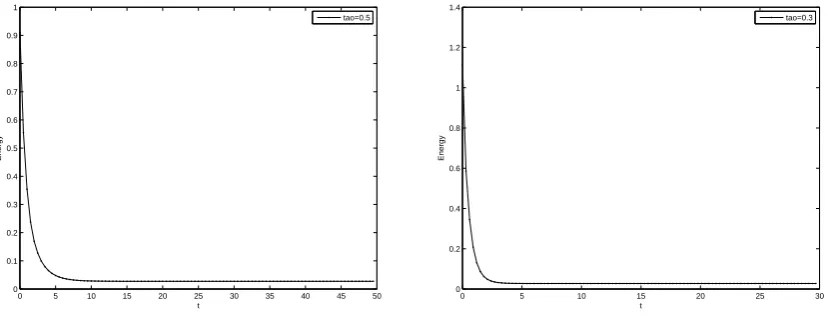
0 5 10 15 20 25 30 35 40 45 50

0 0.1 0.2 0.3 0.4 0.5 0.6 0.7 0.8 0.9 1

t

Energy

tao=0.5

0 5 10 15 20 25 30

0 0.2 0.4 0.6 0.8 1 1.2 1.4

t

Energy

tao=0.3

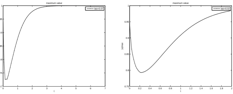
0 1 2 3 4 5 6 7 0.7

0.75 0.8 0.85 0.9 0.95 1

t

|u|max

maximum value

tao=0.07

0 0.2 0.4 0.6 0.8 1 1.2 1.4 1.6 1.8 2 0.75

0.8 0.85 0.9 0.95 1

t

|u|max

maximum value

tao=0.02

Fig. 3: Maximum values for scheme (2.18) with time step τ= 0.07, 0.02.

0 1 2 3 4 5 6 7

0 0.2 0.4 0.6 0.8 1 1.2 1.4

t

Energy

tao=0.07

0 0.2 0.4 0.6 0.8 1 1.2 1.4 1.6 1.8 2 0

0.2 0.4 0.6 0.8 1 1.2 1.4

t

Energy

tao=0.02

Fig. 4: Energy for scheme (2.18) with time stepτ = 0.07, 0.02.

Fig1 and Fig3 plots the numerical solution of the discrete scheme (2.18) does not satisfy the maximum principle when the time step is τ = 0.5 or τ = 0.3, but it satisfies the maximum principle when the time step is τ = 0.07 and τ = 0.02. Moreover, Fig2 and Fig4 plots the discrete energy diminishing stability.

Second, we let the parameter 2 = 0.0001 , and the mesh size in space is h = 0.01. We have

1 6 < τ <

5

0 5 10 15 20 25 30 35 40 45 50 0.92

0.93 0.94 0.95 0.96 0.97 0.98 0.99 1 1.01

t

|u|max

maximum value

tao=0.5

0 2 4 6 8 10 12 14 16 18 20

0.88 0.9 0.92 0.94 0.96 0.98 1

t

|u|max

maximum value

tao=0.2

Fig. 5: Maximum values for scheme (2.18) with time stepτ= 0.5, 0.2.

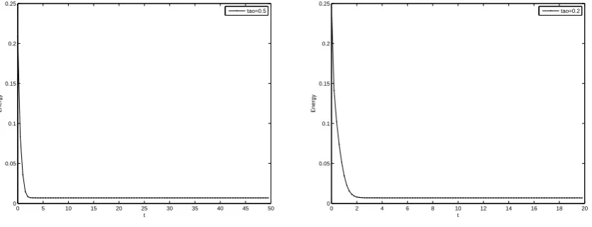
0 5 10 15 20 25 30 35 40 45 50

0 0.05 0.1 0.15 0.2 0.25

t

Energy

tao=0.5

0 2 4 6 8 10 12 14 16 18 20

0 0.05 0.1 0.15 0.2 0.25

t

Energy

tao=0.2

Fig. 6: Energy for scheme (2.18) with time step τ= 0.5, 0.2.

Fig5 plots the numerical solution of the discrete scheme (2.18) does not satisfy the maximum principle when τ = 0.5, but it satisfies the maximum principle when the time step is τ = 0.2. Fig6 plots the discrete energy diminishing stability.

6

Conclusions

The main contribution of this work is the establishment of the full-discrete fourth-order compact difference scheme for the one-dimensional nonlinear Allen-Cahn equation (2.18). For the fully discretized scheme, we prove that the numerical solution is bounded by the constant 1, i.e. numerical maximum principle. This offers us the possibility to achieve the numerical solution satisfies energy stability. At the same time, the restrictions of the step ratio and the time step 1₆ ≤ λ≤ 5₆ , 0 < τ ≤ min{λ− 1₆,1− 6₅λ} are obtained. Finally, the compact difference scheme is considered as a illustrative example to show the effectiveness and advantages of the proposed scheme.

Acknowledgment

Reference

[1] Jiaqi Zhang, Tianliang Hou. Discrete Maximum Principle and Energy Stability of Finite Dif-ference Methods for One-dimensional Allen-Cahn Equations [J]. Journal of Beihua University, 2016.4, 17(2):159-164.

[2] Tao Tang, Jiang Yang. Implicit-Explicit Scheme for the Allen-Cahn Equation Preserves the Maximum Principle [J]. Journal of Computational Mathematic, 2016, 34(5):451-461.

[3] Nan Zheng, Shuying Zhai, Zhifeng Weng. Two Efficient Numerical Schemes for the Allen-Cahn Equation [J]. Advances in Applied Mathematics, 2017, 6(3):283-295.

[4] T.Hou, K.Wang. Discrete Maximum-Norm Stability of A Linearized Second-Order Finite Difference Scheme for Allen-Cahn Equation. Numerical Analysis and Applications, 2017, 10(2):177-183.

[5] Tianliang Hou, Tao Tang, Jiang yang, Numerical Analysis of Fully Discretized Crank-Nicolson Scheme for Fractional-in-Space Allen-Cahn Equations [J]. J Sci Comput,2017, 72:1214-1231.

[6] Tingting Li. Spectral methods for the Allen-Cahn equation and Cahn-Hilliard equation. Huazhong University of Science and Technology, 2015.

[7] Lingling Xu. Second Order Dissipative Difference Scheme for Neumann Boundary Value Prob-lem of Allen-Cahn Equation [D]. Shanghai Jiaotong University, 2010.

[8] Chunli Yu. Local Discontinuous Galerkin Finite Element Method for Allen-Cahn Equation [D]. Shandong University, 2009.

[9] X.B.Feng, A.Prohl. Numerical Analysis of the Allen-Cahn Equation and Approximation for Mean Curvature [J]. Numer Math, 2003, 27(99):33-65.

[10] Jie Shen, Xiaofeng Yang. Numerical Approximations of Allen-Cahn and Cahn-Hilliard Equa-tions [J]. Discrete and Continuous Dynamical Systems, 2010, 28(4):1669-1691.

[11] Yibao Li, Hyun Geun Lee. An Unconditionally Stable Hybrid Numerical Method for Solving the Allen-Cahn Equation [J]. Computers and Mathematics with Applications, 2010, 60:1591-1606.