Article
Modeling Parallel Robot Kinematics for 3T2R and
3T3R Tasks using Reciprocal Sets of Euler Angles
Moritz Schappler1,∗, Svenja Tappe1and Tobias Ortmaier1
1 2 3 4
5 6 7 8
9
10
1 InstitutfürMechatronischeSysteme,LeibnizUniversitätHannover; [email protected]
* Correspondence:[email protected];
Abstract: Industrial manipulators and parallel robots are often used for tasks like drilling or
milling, that require three translational, but only two rotational degrees of freedom (“3T2R”). While kinematic models for specific m echanisms f or t hese t asks e xist, a g eneral k inematic m odel for parallel robots is still missing. This paper presents the definition of the rotational component of kinematic constraints equations for parallel robots based on two reciprocal sets of Euler angles for the end-effector orientation and the orientation residual. The method allows to completely remove the redundant coordinate in 3T2R tasks and to solve the inverse kinematics for general serial and parallel robots with the gradient-descent algorithm. The functional redundancy of robots with full mobility is exploited using nullspace projection.
Keywords: Parallel robot; five-DoF t ask; 3 T2R t ask; f unctional r edundancy; t ask redundancy;
redundancy resolution; reciprocal Euler angles; inverse kinematics
11
1. Introduction
12
Industrial tasks like welding, gluing, milling or drilling represent a major part the of applications
13
of industrial robots, which generally have full mobility, i. e. the operational space of their end-effector
14
has three translational and three rotational (“3T3R”) degrees of freedom (“DoF”). Parallel robots like
15
the Stewart-platform have especially been proposed for milling tasks regarding their high structural
16
stiffness. The task space of the named applications can be defined by three translational DoF and only
17
two rotations due to a symmetry around the tool axis (“3T2R”). This results in a functional or task
18
redundancy, which is not exploited to full extend yet forparallelrobots.
19
1.1. Inverse Kinematics and Resolution of Task Redundancy for Serial Robots
20
Various general gradient-based methods exist to solve the inverse kinematics forserialrobots;
21
either by augmenting the joint space [1] or by reducing the task space [2–5]. The different approaches
22
each define a residual vector and a gradient matrix considering the properties of 3T2R tasks, e. g. by
23
adding a virtual joint axis [1], orthogonal decomposition of the task space [2], rotation of the residual
24
into a task frame and removing the corresponding component [4], defining the tool axis by two points
25
for constructing a nullspace [3] or by defining the absolute orientation and the orientation residual with
26
two reciprocal sets of Euler angles [5]. The gradient matrices corresponding to the different residuals
27
are used for an iterative Newton-Raphson algorithm [6,7] by exploiting the functional redundancy
28
with a null space projection of additional performance criteria [6]. Without the definition of a proper
29
gradient, a global optimization has to be performed outside of the inverse kinematics algorithm [8,9].
30
1.2. Overview of Parallel Robots Structures for 3T2R tasks
31
Parallel robots in 3T2R tasks can be ordered in classes according to their kinematic structure into
32
I mechanisms with full platform mobility (3T3R) that are redundantly controlled to five DoF,
33
II mechanisms with 3T2R platform mobility enforced with a passive five-DoF constraining leg and
34
five other legs with six DoF each,
35
III mechanisms with 3T2R platform mobility resulting from the mobility of five actuated legs with
36
five or six DoF each,
37
IV mechanisms with 3T2R platform mobility and five legs with only five DoF each.
38
The classes I and II were introduced in [10], where class IV is analyzed regarding leg symmetry
39
and singularities. Class III is mainly influenced by the systematic synthesis of [11] and several existing
40
prototypes and is demarcated against class II by the absence of the passive constraining leg. Class
41
IV can be seen as a subclass of III, but is differentiated in this paper due to its characteristics. Other
42
classifications are provided e. g. by [12], where IV and II are termed “families”.
43
Examples for the first class are hexapods1 (6UPS) [13] or the Eclipse [14] machine tool
44
(2PPRS-PPRS). Any other parallel robot with full mobility (see e. g. [11,15,16]) may be used as well.
45
The second class allows for more variety, since the six-DoF mechanism and the five-DoF
46
constraining leg can manifest in different kinematic structures: The UPS structure is used for the
47
six-DoF part of the mechanism by [17] with a focus on kinematic analysis of 5UPS/US, by [18]
48
with a focus on kinetostatic modeling at the example of 5UPS/RUU (see Fig.1a), by [19] with focus
49
on trajectory control of 5UPS/PRPU and by [20] for pose measurement with the passive leg of
50
5UPS/PRPU. Other possible general base structures are RUS at the 5RUS/US example in [17], PUS,
51
which has been investigated for the control of a redundantly actuated 6PUS/UPU regarding the control
52
of the redundant leg with inverse-dynamics control [21] or force control [22].
53
The most-straightforward member of the third class is the 4UPS-UPU of Fig.1b, which is
54
investigated in [23] for a simulation and feasibility study together with a survey on possible
55
architectures for a technical realization of this class. Other possible structures are the 4URS-URU, which
56
is analyzed kinematically in [24] and the 4PSU-PU*U, which has a special parallelogram structure in
57
one leg (termed “U*”) and is presented in [25]. A sub-class of III consists of mechanisms [26–28], where
58
the last joint axis of the legs is coaxial with the tool axis and is constructed as rotating ring. It contains
59
the Metrom machine tool (4SPRR-SPR), depicted in Fig.1c, which is analyzed regarding inverse
60
and forward kinematics in [26] or its variants, the redundant 4SPRR-PSPR from [28] or the hybrid
61
4URHU-URHR with an additional linear actuator at the platform [27]. A structural synthesis based
62
on linear transformations and evolutionary morphology [11] led e. g. to the Isoglide5 mechanisms
63
(3PRRRRR-2PRRRR), which are analyzed and optimized regarding the isotropy of the Jacobian in [29].
64
The simplest member of class IV, the 5UPU is shown in [30] with the help of screw theory to
65
only have local mobility and no global mobility, since the twist systems of the leg chains have no
66
intersection and the resulting twist system of the platform is empty. Members of class IV have been
67
found by systematic structural synthesis with screw theory, which has been performed in [31] for
68
symmetric 3T2R mechanisms. The resulting 5RPUR of Fig.1d and 5PRUR are analyzed in [10,32].
U
P
R
R P U R
P U
S
U U
P S
U S
P R
R
R P S
(a) 5UPS/RUU (class II) (b) 4UPS-UPU (class III) (d) 5RPUR (class IV) U
(c) 4SPRR-SPR (Metrom, class III)
Figure 1.Typical mechanisms of the different classes. Taken from [18] (a), [23] (b), [28] (c), [10] (d).
69
1 The joint structure is denoted by the number of the legs and the order of universal (“U”), prismatic (“P”), spherical (“S”),
In a practical application with competing requirements on workspace, stiffness, costs and
70
precision, each of the existing systems has its legitimization. Nevertheless, each of the classes has
71
inherent disadvantages: In tasks like milling with high process forces and requirements on stiffness
72
and precision, robots from class II with one constraining leg have the drawback, that the passive
73
leg takes the complete reaction wrench in the blocked rotational degree of freedom, which strongly
74
affects the mechanisms stiffness in this direction [18]. The same is argued by [27] at the example of
75
the Metrom machine tool, but can be extended to all the members of class III, where most leg chains
76
have six DoF and usually only one leg chain has five DoF. This leg chain also has to take the reaction
77
moments in the blocked DoF which affects the overall stiffness. Therefore members of the classes
78
I and IV can be expected to reach a higher stiffness. Mechanisms of the class IV may further suffer
79
from an increased sensitivity of manufacturing tolerances, which may cause a high pretension of the
80
bearings or even reduce the DoF, since the five DoF of all leg chains have to coincide exactly to allow
81
the platform to also have five DoF. Additionally, only members of class I provide redundancy which
82
allows to use the additional DoF for performance optimizations e. g. to avoid singularities and to
83
compensate the smaller workspace caused by the sixth leg.
84
Therefore, the remainder of the paper focuses on mechanisms of the first class to allow an
85
optimization of their performance criteria using the degree of task redundancy.
86
1.3. Inverse Kinematics of Parallel Robots for 3T2R Tasks
87
The parallel robots with five DoF presented previously have a kinematic structure, that allows
88
for an analytic model of the inverse kinematics. All references define the end-effector orientation
89
with two consecutive elementary rotations, i. e. define two Euler angles to represent the tool axis
90
orientation in minimal coordinates [10,19–22,26,28,32,33], which is called “partial pose” in [13]. The
91
inverse kinematics problem (IKP) is first solved for the first chain, which is called “leading chain” in
92
this paper. Due to the geometry of the leading chain, this solution can be found algebraically. Then the
93
IKP is solved for the other “following” chains with the given orientation from the leading chain and
94
standard methods. For robots of class II, the constraining leg is selected as the leading leg chain and
95
for class III the 3T2R leg is selected.
96
To the best knowledge of the authors, only one reference [13] for the IKP of functionally redundant
97
parallel robots of the class I is known. The reason presumably is that a solution of the 3T3R IKP for
98
these robots is possible with standard methods, as used in [14] for the 3T3R Eclipse. It is always
99
possible to transfer the 3T2R IKP into 3T3R by adding an arbitrary value for the desired rotation
100
around the tool axis. An optimization of additional performance criteria is possible by varying the
101
redundant rotation angle [8,9]. This approach was chosen in [13] by first defining the IKP with the
102
redundant rotation as a parameter and then performing an optimization of this parameter using
103
analytical computation of the dexterity and interval analysis to ensure a minimum determinant of the
104
inverse Jacobian. The drawback of this method is the need for a cascaded optimization which is more
105
complex than a gradient-based approach presented in this paper.
106
1.4. Motivation and Summary of the State of the Art
107
The overview over the literature shows, that no general, machine-independent methods for the
108
resolution of functional redundancy for 3T3R PKM in 3T2R tasks exists. The works either focus on a
109
general structural synthesis of machines e. g. via screw theory [31] or linear transformations [29] or the
110
description and improvement of specific, manually selected, machines. To choose the best machine for
111
given requirements, a structural synthesis is only the first step. Additionally, a dimensional synthesis
112
should be performed for all possible structures to select the most suitable mechanism. This combined
113
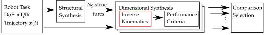
structural and dimensional synthesis [34] is sketched in Fig.2. To be able to perform the dimensional
114
synthesis for all structures, the inverse kinematics has to be implemented in a general form, to calculate
115
the performance criteria over a given trajectory for further optimization of the structures and their
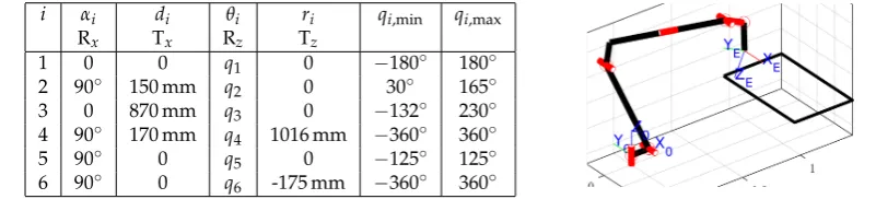
116
comparison. For the generation of task redundant parallel robots, the inverse kinematics has to
Robot Task Structural Synthesis
Dimensional Synthesis Comparison Selection DoF:αTβR
Trajectoryx(t)
.
NS struc-tures
..
Inverse Kinematics
Performance Criteria
Figure 2.Overview of the procedure for combined structural and dimensional synthesis.
include an optimization of the performance criteria and the restrictions such as joint limits, to ensure a
118
comparability of the results. To address this, the contributions of this paper are
119
• a general kinematics model for parallel robots using the concept of reciprocal Euler angles [5],
120
• a complete elimination of the redundant operational space coordinate in this formulation for
121
3T2R tasks allowing a nullspace optimization in the gradient-based inverse kinematics,
122
• proofs, examples and simulations to show the performance for single serial kinematic leg chains
123
and complete parallel robots.
124
The remainder of the paper is structured as follows: The description of the inverse kinematics
125
problem and prior definitions are given in Sec.2and the concept of reciprocal Euler angles from
126
[5] is adapted in Sec.3for parallel robots. This leads to the full kinematic constraints of parallel
127
robots in 3T2R tasks, introduced in Sec.4and applied to the differential kinematics in Sec.5. The
128
theoretical analysis is followed by examples and simulations in Sec.6. The appendix contains proofs
129
and additional details on the mathematical formulation.
130
2. Inverse Kinematics Problem for Parallel Robots
131
Before addressing the specific model for parallel robots in 3T2R tasks in the next section, the standard kinematics model of kinematics of parallel kinematic machines (“PKM”) is repeated in the following, corresponding to the state of the art [11,15,35] and serving as a reference to highlight its shortcomings for 3T2R tasks. The regarded parallel robot consists ofmlegs, which each have the joint coordinatesqi. All joints are considered as single-DoF and additionally to the active jointsqi,a
explicitly all passive joints at the base and at the platformqi,pare included in the coordinatesqiof legi. The coordinates
x=hxTt xTriT∈R6 (1)
of the end-effector platform describe the position and orientation of the end-effector frameFDwith
respect to the base frameF0. In the equations, this is marked with left subscript “(0)” for vectors and left superscript “0” for rotation matrices. The platform-related end-effector frame is the desired frame in the inverse kinematics problem and is therefore abbreviated with “D”. The position
xt=(0)rD∈R3 (2)
is defined as the origin of the platform frame and the rotation matrix
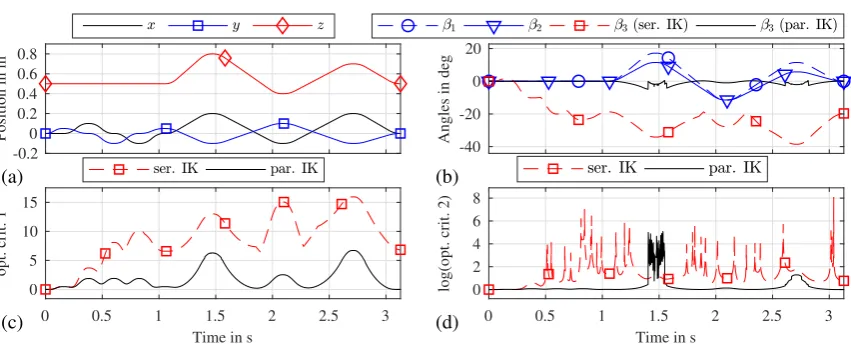
0RD(x r) =
h
nD oD aDi∈SO(3) (3)
of the platform frame is expressed with Euler angles
xr =
h
β1 β2 β3
iT
=:β∈R3 (4)
as a minimal representation of the orientation coordinates. The symbol “β” will be used to denote orientations relative to the base frame throughout this paper. TheX-Y-Z-notation
is used for the Euler angles without loss of generality. The relation between joint coordinates q
and platform coordinatesxis established with the kinematic constraint equations, for which most commonly the vector loop
Φt,i(qi,x) =−(0)rAiBi(x) +(0)rAiBi(qi) (6) between the position of the platform coupling pointBirelative to the base coupling pointAiis used
for each leg chaini[15]. The second term(0)rAiBi(qi)corresponds to the forward kinematics of the serial leg chain. The vector
(0)rAiBi(x) =−(0)rAi+xt+ 0RD(x
r)(D)rBi (7)
includes the term0RD(xr)that depends on the full orientationxrof the end-effector. For the bigger part of existing parallel robots, the passive joint coordinates can be eliminated analytically from the equations (6), e. g. by using the Euclidian distance for UPS or RPR leg chains or via trigonometry for RRR-chains. This is termed “minimal kinematics set” in [15] and leads to the scalar constraint equation
Φi=Φi(qi,a,x) (8)
for each legi, which can be assembled to the vector of constraint equations
Φ(qa,x) =
h
Φ1 Φ2 · · · Φm iT
(9)
for allmlegs of the PKM . The differential kinematics of the PKM is calculated with the time derivative d
dtΦ(qa,x) =Φ∂qaq˙a+Φ∂xx˙ =0 (10)
where the passive joint coordinatesqpdo not occur, since they have been eliminated in a previous step. The inverse-kinematics matrix2
Φ∂qa = ∂Φ
∂qa =
Φ1,∂q1,a 0 0 0
0 Φ2,∂q2,a . .. 0
0 . .. . .. 0 0 0 0 Φm,∂qm,a
(11)
of this model has diagonal form and the direct-kinematics matrix
Φ∂x= ∂Φ
∂x =
∂Φ1/∂x ∂Φ2/∂x
.. . ∂Φm/∂x
(12)
is fully populated. This definition of the constraints has the following drawbacks:
132
1. For parallel robots with arbitrary leg chains like those generated by a structural synthesis
133
[11,31,34], it is generally not possible to analytically eliminate the passive joint coordinates.
134
2. If more than three joint coordinates per leg influence the coupling point positionBi, the three
135
kinematic constraints per joint in (6) are not sufficient to generate enough equations for the
136
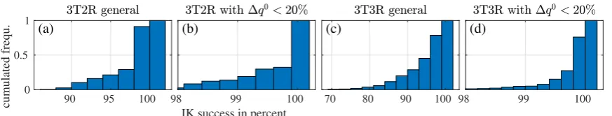
matrix of (11) to become invertible. The velocity-based theory of linear transformations used by
137
2 We follow the argumentation from [11] to avoid the term “Jacobian”, since the matrix is not a Jacobian in the mathematical
[11] allows to determine the mobility of arbitrary parallel robots. The linear transformation is
138
generalized in [12] to accuracy and stiffness modeling by means of screw theory resulting in the
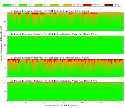
139
“generalized Jacobian”. Both concepts do not provide a direct appliance to solve the IKP, since
140
this requires a formulation of the orientation at position level, not velocity level.
141
3. Exploiting the reduction of end-effector coordinates for 3T2R tasks is not possible, since all
142
end-effector coordinates are included in (7).
143
An alternative kinematic model to encounter the combination of these points is presented in the next
144
section, where the concept of reciprocal sets of Euler angles for the inverse kinematics problem for
145
serial link robots [5] is transferred to the leading leg of parallel robots.
146
3. Reciprocal Sets of Euler Angles for the Kinematics of a Serial Leg Chain
147
To take the rotational symmetry around the tool axis in 3T2R tasks into account, a new set of task space coordinates
η=
h
ηTt ηTr
iT
∈R5 (13)
has to be defined. The translational part
ηt=xt=(0)rD∈R3 (14)
remains unchanged relative to the operational space coordinatesx. The rotational part
ηr =
h
β1 β2
iT =
"
1 0 0 0 1 0
#
| {z }
=Pηr
xr∈R2 (15)
only contains the first two rotational coordinates ofx. The last operational space coordinateβ3, the rotation around thez-axisaDofFD, is excluded from the task space by the selection matrixPηr. To be
able to set the rotational DoF around the tool axis in 3T2R tasks arbitrarily and use gradient-based inverse kinematics,β3has to be eliminated completely from the kinematics equations (6). To simplify the following elaborations, the platform frameFDis still identified as the desired frame of the inverse
kinematics problem and the end-effector frame that results from the joint angles of legiis now termed FE, which corresponds to the forward kinematics of the leg chain. For a formulation without the tool
axis rotation, a different constraint definition
Φt,i(qi,x) =−(0)rD+(0)rE(qi) =−xt+(0)rE(qi)∈R3 (16)
containing the vector loop from the robot base frame F0 to the platform FD and the leg chain
148
end-effectorFEcan be used, where in contrast to (6) only the translational partxtof the end-effector
149
coordinates appears and not the rotational partxr. The vector loop is depicted in Fig.3for a planar
150
robot with opened (Fig.3a, b) and closed loops (Fig.3c). The triangle represents the end-effector
151
platform and only one leg chain is drawn in the figure.
152
r0D(x) r0E(qi)
r0D=r0E E
D
(a) (b) (c)
Φt,16=0 Φr,16=0 Ψr,16=0
Φt,1=0 Φr,16=0 Ψr,1=0
Φt,1=0 Φr,1=0 Ψr,1=0
O Ai
Bi
Ai B Ai
i
Bi
As a drawback of (16), all joint anglesqiof the legiand not only the coordinates of the first joints counted from the base are now included in the vector
(0)rE(qi) =(0)rAi +(0)rAiBi(qi) + 0R
Bi(qi)(Bi)rE. (17)
This implies, that the platform is now part of the last link of the considered leg chain, as sketched in Fig.3by the dashed triangle. To account for the increased number of included joints in (17), the full kinematic constraints
Φi= h
ΦTt,i ΦTr,i
iT
∈R6, (18)
have to be considered, including the rotational part
Φr,i(qi,x) = h
α1 α2 α3
iT
=α
D
RE(xr,qi)
=α
0RT
D(xr)0RE(qi)
, (19)
which is needed to generate enough equations for an invertible matrix in the differential equations.
153
The constraints again contain the deviation between the desired end-effector frameFDexpressed with
154
xand the actual robots end-effector frameFEexpressed withq. Fig.3(b) and (c) show cases, where
155
the translational constraints are met, but the rotational constraints have different values. For 3T3R
156
tasks, only Fig.3(c) represents a valid solution of the inverse kinematics. For 3T2R tasks, Fig.3(b) and
157
(c) represent valid solutions.
158
The goal of eliminating the tool rotationβ3from the equations is not achieved yet, since all three components of the platform orientationxraffect the rotation matrix0RD. This can be addessed by the selection of the Euler angles: Similar to the definition of the rotational operational space coordinatesxr in (4), the constraintsΦr,i are also expressed with a set of Euler anglesα. In the following, “α” will always refer to the rotation error/residual and “β” to an orientation relative to the base frame. The Euler angle convention ofαcan be chosen independently of the choice for the orientation representation inβ. The intuitive approach of choosing
R(α∗):=Rx(α∗1)Ry(α∗2)Rz(α∗3)∈SO(3) (20)
the same way asβleads to a set of transformations depicted in Fig.4(a) where the intermediate steps
159
of the single elementary rotations are omitted since they have no technical meaning. The upperscript
160
asterisk in (20) demarcates this specific example and the following elaborations on the calculation ofα.
161
To be able to remove the redundant coordinateβ3from the rotational constraints of (19), it is necessary to change the expression of the orientation errorαto be reciprocal to the expression of the absolute orientationβ. By using theZ-Y-X-Euler angles with
R(α):=Rz(α1)Ry(α2)Rx(α3)∈SO(3) (21)
only the error componentα1is affected by rotations around the tool axis, which is thez-axis of the intermediate framesFA1,FA2and the platform frameFDin Fig.4(b), where the frame rotations with
F0 FD
Rx(β1)Ry(β2)
FE 0R
E(q1)
Ry(α2)Rx(α3)
FA1
FA2
Rz(α1)
Rz(β3+α1)
Rz(β3)
F0 FD
0R
D(xr) =Rx(β1)Ry(β2)Rz(β3)
FE 0R
E(q1)
Rx(α∗1)Ry(α∗2)Rz(α∗3)
(a) (b)
the reciprocal set of Euler angles are sketched. The mathematical proof is given in appendixA.1and in [5]. The new, reduced rotational part of the kinematic constraints
Ψr,i(qi,η) = h
α2 α3
iT =
=PΨr
z }| {
"
0 1 0 0 0 1
#
Φr,i(qi,x)∈R2 (22)
does not contain the tool rotation any more. The full kinematic constraints for the reduced coordinates
Ψi= h
ΦTt,i ΨTr,i
iT
∈R5 (23)
can be used for the inverse kinematics of the leg chainiin 3T2R tasks, whereΨi=0leads to a valid
162
position and orientation of the tool axis. The conditionΦi =0leads to a valid configuration of legiof
163
the parallel robot in 3T3R tasks. In the following, “Φ” is always used for 3T3R3kinematic descriptions
164
and “Ψ” for 3T2R.
165
4. Full Kinematic Constraints for Parallel Robots using Reciprocal Sets of Euler Angles
166
The definition of the full kinematic constraints (16,19,18) of a single leg chain of the parallel robot from the previous chapter can be used to write the kinematic constraints in a general form. The full kinematic constraint equations can only be defined for 3T3R tasks without further adaptions as
Φ=
h
ΦT1 ΦT2 · · · ΦTm
iT
. (24)
The constraints Ψi from (23) for the reduced coordinatesηcan only be defined for one leg chain:
167
Fig.5(a) show an open-loop second leg chain for a given first leg chain from Fig.3. By also closing
168
the3T2Rkinematic constraintsΨ2for the second loop, as depicted in Fig.5(b), the tool axis stays
169
arbitrary and the platform pose demanded from the two legs would be different and therefore would
170
not be a valid solution for the complete mechanism, i. e.Φ26=0. Only if the second leg fulfills the
171
3T3Rkinematic constraints for all platform coordinates, as shown in Fig.5(c), a valid configuration
172
of the mechanism emerges. This approach has already be used for many specific robots systems, as
173
introduced in Sec.1. As a generalization, the first leg of the parallel robot is now termed the “leading
174
leg chain” (Index “1”) and the other legs are termed as “following leg chains” (Index “j”).
175
The translational part of the constraints is not coupled by the platform orientation and therefore left unchanged relative to (16) with
Φt,j(qj,x) =−(0)rD+(0)rE(qj) =−xt+(0)rE(qj)∈R3 (25)
3 By omitting the corresponding lines in the operational space coordinatesxand the constraint equationsΦ, it is also possible
to use the 3T3R approach for systems with reduced mobility of 2T1R, 3T0R and 3T1R platform DoF.
(a) (b) (c)
L
r0L(q1)
r0E(q2)
E
O Φt,26=0
Φr,26=0 Ψr,26=0
Φt,2=0 Φr,26=0 Ψr,2=0
Φt,2 =0 Φr,2 =0 Ψr,2 =0
for the following legsj. The orientation for the platform is given with the rotation matrix 0RL(q
1):=0RE(q1) (26)
which gives the reference end-effector frameFLresulting from the leading leg 1. The rotational part of
the kinematic constraints
Φr,j(qj,q1) =α(0R T
L(q1)0RE(qj)) (27)
for the following leg is given by the Euler angle representation of the deviation between the orientation of the platform frameFLgiven by the leading (“L”) leg and the frameFEgiven by the respective
following legj. The choice of the Euler angle notation is arbitrary. The full kinematic constraints for the complete parallel robot withmlegs for 3T2R tasks
Ψ=
h
ΨT1 ΦT2 · · · ΦTm
iT
(28)
are assembled from the 3T2R constraintsΨ1from (23) for the leading leg and the 3T3R constraints
176
Φj, 2≤j≤mfrom (25,27) for the following legs. The index “j” is used to distinguish the following
177
legs of the 3T2R case and all legs “i” of the general case in Sec.3. The full constraints of (28) lead
178
to a 35-dimensional vector for the kinematic constraints for parallel robots with six legs in 3T2R
179
tasks, which are aggregated as class I in Sec.1.2. This formulation can be reduced by combining the
180
mechanism-specific approach for the constraints from (6) with the principle of leading and following
181
legs of this section. For the 6UPS structure this would result in a 10-dimensional constraint vector with
182
five entries for the leading leg and only one entry for each following leg.
183
5. Differential Kinematics for Parallel Robots
184
To be able to compute the differential kinematics of the constraintsΦ(24) andΨ(28) to
d
dtΦ(q,x) =Φ∂qq˙+Φ∂xx˙ =0 and d
dtΨ(q,η) =Ψ∂qq˙+Ψ∂ηη˙ =0, (29)
the full geometric matrices of inverse kinematics
Φ∂q(q,x) =
Φ1,∂q1 0 0 0
0 Φ2,∂q2 . .. 0 ..
. . .. . .. 0
0 0 0 Φm,∂qm
and Ψ∂q(q,η) =
Ψ1,∂q1 0 0 0
Φ2,∂q1 Φ2,∂q2 . .. 0 ..
. . .. . .. 0 Φm,∂q1 0 0 Φm,∂qm
(30) and the full geometric matrices of direct kinematics
Φ∂x(q,x) = ∂Φ
∂x =
Φ1,∂x
Φ2,∂x .. . Φm,∂x
and Ψ∂η(q,η) =
∂Ψ
∂η =
Ψ1,∂η
Φ2,∂η
.. . Φm,∂η
(31)
have to be calculated for the 3T3R and the 3T2R case respectively. The gradientΦ∂qhas block diagonal
185
form, indicating that the inverse kinematics problem can be solved for each leg independently. The
186
structures of the gradientΨ∂q results from the coupling of the leading and following joints in the
187
rotational constraints equation.
188
The gradient matricesΦ∂qandΦ∂xcontain nested nonlinear functions related to the orientation
189
error, therefore the geometric Jacobian of the leg chains can not be exploited for the rotational part, as
190
derived in appendixA.2. The gradients are calculated with the chain rule and a syntax for stacking
matrix columns to avoid differentiating matrices or with respect to matrices, which was introduced
192
in [5]. The product operatorΠ, the stacking operatorRand the transpose operatorPTused for the
193
implementation in the next section are explained in appendixA.3.
194
5.1. Constraint Gradients for the Leading Leg of the 3T2R and all Legs of the 3T3R case
195
The constraint definitionΨ1for the leading leg of the 3T2R case (28) andΦiwithi=1, ...,mfor
all legs of the 3T3R case (24) are subject to the same model of (16,19,18). In the following, the 3T3R constraints are displayed. The formΨ1for the 3T2R case is obtained by removing the corresponding line of the rotational component according to (22) and replacing “Φ” by “Ψ” in the following equations. For the analysis, the constraint gradient matrix w. r. t. the joint coordinates has to be divided out to
Φ1,∂q1 = h
ΦTt,1,∂q
1 Φ
T r,1,∂q1
iT
, (32)
where the translational component can be calculated with the geometric Jacobian of the leg chain, as
196
derived in appendixA.2. The rotational part is written down as a function composition of the three
197
functionsα(Euler angles),∏(matrix product) and0RE(rotation matrix) as
198
Φr,1,∂q1 = ∂
∂q1α
0RT
D(x)0RE(q1)
= ∂
∂q1α
∏
0RT
D(x),0RE(q1)
, (33)
which is then expanded with the chain rule for differentiation and the stack operators to
Φr,1,∂q1 = ∂α
∂R
|{z}
I∈R3×9 ∂∏
0RT
D,0RE
∂0RE
| {z }
II∈R9×9
∂0RE(q1)
∂q1
| {z }
III∈R9×dim(q1)
∈R3×dim(q1). (34)
The two first partial derivatives from (34) are sparse matrices and can be calculated efficiently as shown in appendixA.3. The factor “I” contains (A20) withR=DRE(xr,q1)and the factor “II” is (A23) with the contents of0RTD(xr). The last partial derivative “III” can be derived with computer algebra systems from the analytic expression of the rotation matrix0RE(q1). The leading legs constraint gradient matrix w. r t. the platform coordinates can be expanded in the same manner into
Φ1,∂x= "
Φt,1,∂xt Φt,1,∂xr
Φr,1,∂xt Φr,1,∂xr #
= "
−1 0
0 Φr,1,∂xr #
, (35)
where the definitions from (16) and (19) only leave the rotational part
Φr,1,∂xr= ∂
∂xrα
0RT
E(q1)0RD(xr)
T
= ∂
∂xrα
PT
∏
0RT
E(q1),0RD(xr)
(36)
= ∂α
∂R
|{z}
I∈R3×9
PT
|{z}
II∈R9×9 ∂∏
0RT
E,0RD
∂0RD
| {z }
III∈R9×9
∂0RD(xr)
∂xr
| {z }
IV∈R9×3
∈R3×3,
where the simplicity of the single expression “I”-“IV” is demonstrated in appendixA.3. The factors are
199
(A20) withR=DR
E(xr,q1)in “I”, the permutation matrix for transposition from (A19) in “II”, (A23),
200
where the contents of0RT
Eare inserted in “III” and (A21) with the elements ofxrforβin “IV”.
201
5.2. Constraint Gradients for the Following Leg in the 3T2R Case
202
3T2R case, the gradientsΦj,∂q1,Φj,∂qj andΦj,∂xwithj =2, ...,mfrom the right part of (30) and (31)
have to be calculated in a similar way. Due to the abscence of the platform orientation in (27), (35) simplifies for the following leg to
Φj,∂x=
"
−1 0
0 0
#
. (37)
The gradient w. r. t. the joint coordinates of the following leg contains again the translational part of the legs Jacobian regarding the end-effector platform position inΦt,j,∂qj and has the rotational part
Φr,j,∂qj = ∂
∂qjα
0RT
L(q1)0RE(qj)
= ∂
∂qjα
∏
0RT
L(q1),0RE(qj)
(38)
= ∂α
∂R
|{z}
I∈R3×9 ∂∏
0RT
D,0RE
∂0RE
| {z }
II∈R9×9
∂0RE(qj)
∂qj
| {z }
III∈R9×dim(qj)
∈R3×dim(qj),
which is similar to the expression in (34). The factors of the equation (38) are (A20) withR=LRE(q1,qj)
in “I”, (A23), where the elements of0RTL(q1)have to be inserted in “II” and the partial derivative of the platform orientation calculated from legjw. r. t. the legs joint coordinates in “III”, similar to term “III” from (34). The gradient w. r. t. the joint coordinates of the leading leg
Φr,j,∂q1 = ∂
∂q1α
0RT
E(qj)0RL(q1)
T
= ∂
∂q1α
PT
∏
0RT
E(qj)0RL(q1)
(39)
= ∂α
∂R
|{z}
I∈R3×9
PT
|{z}
II∈R9×9 ∂∏
0RT
E,0RL
∂0RL
| {z }
III∈R9×9
∂0RL(q1)
∂q1
| {z }
IV∈R9×dim(q1)
∈R3×dim(q1).
is similar to the expression in (36). The order of the residual expression (27) has to be switched
203
by exploiting the associative property of matrix transposition to avoid differentiating a transposed
204
matrix. The factors of equation (39) are (A20) withR=LRE(q1,qj)in “I”, the permutation matrix for
205
transposition from (A19) in “II”, (A23) with0RT
E(qj)in “III” and the term “III” from (34) in “IV”.
206
5.3. Gradient-Based Solution of the Inverse Kinematics Problem with Redundancy Resolution
207
The presented kinematic constraints and their gradient matrices can be used to solve the inverse kinematics problem (IKP) of single leg chains and complete parallel robots. Since all active and passive joint angles are involved for the case of parallel robots, solving their IKP results in solving the IKP for all leg chains. As first introduced in [7] for Euler angle residuals in the IKP, the Taylor series expansion ofΦ(q,x)leads to the definition of
Φ(qk+1,x) =Φ(qk,x) + ∂
∂qΦ(q,x)
qk
(qk+1−qk) (40)
in an iterative algorithm at the stepk+1, which can be used to solve the IKP using a given initial valueq0and the condition
Φ(qk+1,x) =0. (41)
Defining the solution of the IKP as the main task (“T”), the step-wise solution for the joint coordinates results to
Depending on the dimension, (·)† denotes the matrix inverse or the pseudo-inverse. Again, the
208
equations (40-42) can be written with “Ψ” from (28) instead of “Φ” from (24) for the 3T2R case.
209
In the latter case, the corresponding gradient matrixΨ∂q(q,η)from (30) allows the definition of a nullspace in the case of dim(q1) > dim(η). This redundancy can be exploited by using the nullspace (“N”) projection∆qNfrom [6] additionally to the solution∆qTof the IKP in (42) with the new increment
∆qk=qk+1−qk=∆qTk+∆qkN =−Ψ†∂qΨ+ (1−Ψ†∂qΨ∂q)h∂q (43) in the iterative algorithm. The optimization of additional performance criteriahrequires their gradient h∂qw. r .t the joint positions. One criterion is the summedW1-weighted quadratic distance
h1(q) = 1 2(q−q¯)
TW
1(q−q¯), h1,∂q= ∂h1
∂q =W1(q−q¯) (44)
of the joint positionsqfrom their respective reference position ¯q, e. g. used in [2,36]. Defining ¯qto be in the middle of the joint limits and minimizingh1(q)reduces the risk of joints reaching their technical limits, but does not guarantee it, since exceeding the limit for one joint can be compensated by improving other joints. TheW2-weighted hyperbolic joint limit distance
h2(q) = 1 n
n
∑
i=1
w2,i
(qi,max−qi,min) 8
1
(qi−qi,min)2
+ 1
(qi−qi,max)2
(45)
from [8] (written element-wise forn=dim(q)) circumvents this problem by generating infinitely high values when reaching the limits. In contrast toh1, the criterionh2is only defined for joints within their limits withqi,min<qi<qi,max, which is ensured by settingw2,i =0 for joints exceeding their limits
andw2,i =1 otherwise. To combine the effect of drawing joint positions to their middle withh1of (44) and of strongly rejecting joints directly near their limits withh2of (45), their weighted sum
h3(q) =Kh1h1(q) +Kh2h2(q) (46)
is used in the simulation studies of Sec.6. Other criteria not related to the joint limits are for example
210
stiffness [9] or singularity avoidance via Frobenius-norm condition number [8] or squared condition
211
number [3]. The method can be used for serial link robots as well by removing all entries for the
212
following legs from the formulas, as presented in [5]. The platform posex/ηcorresponds to the desired
213
pose for the serial robots end-effector and the kinematic constraintsΦ/Ψcorrespond to the residual of
214
the IKP.
215
In the practical implementation, it has proven to be useful to extend the basic principle of (43) to
∆qk =KLim(qk)KRel(qk)(KT∆qkT+KN∆qkN), (47)
where the constant damping coefficients KT for ∆qkT and KN for ∆qkN were introduced to avoid
216
overshooting of the solution for the prize of slower convergence. The damping term KN has to
217
be chosen according to the optimization criterion. Further damping was introduced for the 3T2R
218
case with task redundancy to reduce a∆qkthat would lead to overshoot over the joint limits with
219
KLim(qk). The valueKLim =1 is set if no limits would be violated by the increment∆qk. For the 3T3R
220
case,KLim:=1 is set permanently, since slowing down when approaching the limits does not change
221
the direction of the increment and violating the limits is inevitable. The maximum step size for one
222
iteration∆qkwas ensured withKRel(qk)to stay below 5 % of the joint limit range to prevent leaving the
223
validity of the first-order linearization of (40). For smaller increments,KRel =1 holds. The damping
224
terms are always applied to the full vector and not to single elements and therefore only change the
225
norm and not the direction of∆qk.
5.4. Differential Kinematics for the Parallel Robot and its Applications
227
The reasonings so far only considered the inverse kinematics of the parallel robot. The kinematic definitions can also be used in the differential kinematics (29) to establish the connection between joint and platform velocity. This was already presented in general form in [15] and also corresponds to the theory of linear transformation which is the base of the works of Gogu on structural synthesis [11]. The derivation in this paper is based on the positionandorientation, but comes to the same result as the already-existing velocity-based approach. Further, usingΨ/ηas elaborated before allows for the first time to define differential kinematics specifically for 3T2R tasks in a general form. The differential equation of (29) is expanded to
d
dtΦ(qa,qp,x) =Φ∂qaq˙a+Φ∂qpq˙p+Φ∂xx˙ =0 (48)
to distinguish active (“a”) and passive (“p”) joints. The latter also contain the coordinates of the platform-connecting joints. Reordering the equation leads to the full inverse differential kinematics
Φ∂xx˙ =− h
Φ∂qa Φ∂qp i
"
˙
qa
˙
qp #
=Φ∂ap
"
˙
qa
˙
qp #
,
"
˙
qa
˙
qp #
=−Φ−∂ap1Φ∂xx˙, (49)
which has been adressed in the previous sections, and the full direct differential kinematics
Φ∂qaq˙a=−
h
Φ∂x Φ∂qp i
"
˙
x
˙
qp #
=Φ∂xp
"
˙
x
˙
qp #
,
"
˙
x
˙
qp #
=−Φ−∂x1pΦ∂qaq˙a. (50)
By only selecting the first rows for ˙qain (49) and for ˙xin (50), the well-known analytic Jacobian4of the
228
parallel robot [11,15], relating actuator velocities ˙qaand platform velocities ˙x, can be obtained from
229
both equations. For the case of task or kinematic redundancy, the pseudo-inverse can be used forΦ∂ap
230
in (49) as shown in Sec.5.3. The case of task redundancy does not affect (50), since the full platform
231
velocity ˙xis obtained from given actuator velocities ˙qa.
232
6. Results
233
To evaluate the inverse kinematics algorithm presented in the previous section5.3, first the
234
solution of the IKP is shown for the trajectory of a serial-link industrial robot in Sec.6.1and for the
235
trajectory of a parallel robot in Sec.6.2. The results are generalized by the statistical analysis of random
236
point-to-point movements of arbitrary serial link chains in Sec.6.3.
237
6.1. Resolution of Functional Redundancy of a Serial-Link Six-DoF Robot in 3T2R tasks
238
The first evaluation of the inverse kinematics algorithm from Sec.5.3 is performed with
239
simulations at the basic example of a six-DoF industrial robot with a rectangular trajectory. The
240
manipulator Fanuc M-710 iC/50 was taken from the example of [36] with the tabulated kinematics
241
parameters and a sketch of the trajectory in Fig.6. Deviations in the parameters relative to [36] result
242
from the use of themodifiedDenavit-Hartenberg5notation for the joint transformation according to
243
KHALILand the use of only positiveαiparameters for axis alignment for consistency with the results
244
of the structural synthesis from [34]. The trajectory is a rectangle with 500 mm×800 mm and a desired
245
alignment of thez-axis pointing into the ground plane.
246
4 This matrix is related to the time derivatives ˙xrof the platform Euler angles and is called “design Jacobian” in [11] and
“Euler angles inverse jacobian matrix” in [15] in contrast to the Jacobian related to angular velocities of the platform.
5 The four DH parameters contain the minimal set of kinematic parameters for single joint transformations which correspond
i αi di θi ri qi,min qi,max Rx Tx Rz Tz
1 0 0 q1 0 −180◦ 180◦
2 90◦ 150 mm q2 0 30◦ 165◦ 3 0 870 mm q3 0 −132◦ 230◦ 4 90◦ 170 mm q4 1016 mm −360◦ 360◦ 5 90◦ 0 q5 0 −125◦ 125◦ 6 90◦ 0 q6 -175 mm −360◦ 360◦
Figure 6.Left: Table with the kinematic parameters of the industrial manipulator Fanuc M-710 iC/50. Right: sketch of the robot scenario.
The IKP is solved with two settings: Setting the tool axis rotation to different constant valuesβ3
247
with the 3T3R algorithm and solving the IKP only for the desired pointing direction with the 3T2R
248
algorithm. The algorithm from (43) was used in the extended version of (47) for both cases with
249
different settings caused by their nature. For the 3T3R case,KT=0.7 andKN =0.7 were set. The terms
250
KNandKLimhave no effect, since no nullspace movement is possible. For the 3T2R case, withKh1 =0
251
andKh2 =1 only the hyperbolic limit rejection criterion from (45) was used. The first criterion was not
252
used, since in the trajectory example the limits are not even temporarily exceeded by principle. All
253
IKP algorithms had the same initial value from Fig.6.
254
The results of the inverse kinematics for different settings are given in Fig.7, where the
255
representative joint coordinatesq1andq5, the redundant coordinate of the end-effector orientation
256
β3, as well as the optimization criterion (45) are depicted over time for the trajectory from Fig.6. The
257
positions are normalized to the joint limits from -1 to 1. The first three lines in Fig.7represent IKP
258
solutions with a given constant end-effector orientation β3 of−150◦,−15◦ and 45◦ and the 3T3R
259
algorithm. The 3T2R algorithm without nullspace optimization is plotted with dotted lines for each
260
first sample of the 3T3R cases as initial value with the same colors. Using these initial values for a
261
3T2R IK with optimization leads to strong nullspace movements at the beginning, quickly converging
262
to a local minimum. Therefore the 3T2R case with optimization, plotted as the green line with triangle
263
markers, is shown only for the initial condition from Fig.6. It can be observed, that the optimization
264
of the criterion leads to the best solution of the IKP. The lines for the criterion forβ3 = −150◦and
265
β3=−15◦partly exceed the limits of the plot, indicating that the limit is violated, which can also be
266
seen at the plot forq5. This exposes the need for keeping the solution always within the limits by the
267
measures described. The 3T2R IK without optimization with dotted lines tends to lower changes in the
268
joint positions than the 3T3R IK, since this corresponds to the solution of the matrix pseudo-inverse in
269
(43).
270
0 2 4
Time in s -0.3
-0.2 -0.1 0 0.1 0.2
0 2 4
Time in s -1
-0.5 0 0.5 1 1.5
0 2 4
Time in s -200
-150 -100 -50 0 50 100 150
0 2 4
Time in s 1
2 3 4 5 6 7
6.2. Resolution of Functional Redundancy of a Parallel Robot in 3T2R tasks
271
As elaborated in Sec.4and5, the solution of the IKP for 3T2R and 3T3R tasks is necessary to solve
272
the problem for parallel robots. Therefore the trajectory evaluation for a 6UPS parallel robot6in this
273
section is preceded by the trajectory example for a serial link chain in the previous section. This robot
274
belongs to the first class presented in Sec.1.2, which is primarily addressed in this paper.
275
The robot has a Gough-structure [15] with symmetric alignment of the universal joint base
276
couplings on a circle with radiuskr0Aik=1 m and the spherical joint platform couplings on a circle
277
with radiuskrBiEk=0.4 m. The initial pose was set to a center positionxTt = [0, 0, 0.5 m]and the initial
278
orientationxrwas set to zero, meaning an alignment of base and platform frame. The joint positions
279
for each leg were defined to have the initial valuesqT
i = [30◦,−30◦, 0.583 m, 0◦, 30◦, 60◦]for the given
280
initial platform pose to avoid switching±πwithin the trajectory and to avoid gimbal-lock-singularities.
281
The joint limits were set around the resulting zero position to±0.5 m for the prismatic joint and±60◦
282
for all single revolute joints representing the universal and spherical joints. The values are higher than
283
typical values for real robots to emphasize the effect of the nullspace movement in a bigger simulated
284
workspace of the robot. The settings for the IK solver are similar as in Sec.6.1, since both cases regard
285
solving the IKP for a trajectory.
286
The time evolution of platform pose and optimization criteria is depicted in Fig.8. The reference
287
trajectory can be seen at the platform position in Fig.8a and the platform orientation expressed in
288
X-Y-Z-Euler angles (β1-β3) relative to the base frame in Fig.8b. The IKP is solved using two different
289
methods: Only solving the IKP for the legs separately, called “ser. IK” in Fig.8and solving the IKP
290
for all legs together, called “par. IK” in Fig.8. Both methods perform an optimization with onlyh2of
291
(45), as justified in Sec.6.1. The first approach only performs this optimization according to Sec.3for
292
the first leg using the 3T2R method and then solves the IKP for all other legs with the 3T3R method.
293
The second approach uses the optimization for all legs together according to the 3T2R method from
294
Sec.4. This results in improved values for the performance criteria depicted forh1in Fig.8c and forh2
295
in a logarithmic scale in Fig.8d. Since the first approach does not regard the limits of the following
296
legs, the optimization criterion gives high values indicating many joint limit violations. The second
297
approach only shows peaks att=1.5 s in Fig.8d that result from a joint position getting near to the
298
limit, but not exceeding it. For the practical implementation, the computation time is only weakly
299
influenced by the selection of the method, since calculating the (pseudo)-inverse for six 5×6 and 6×6
300
or one 35×36 matrices does not present a challenge for current computing hardware. Therefore the
301
“par. IK”-method should be preferred.
302
6 For solving the full IKP, the actuation (such as “6UPS”) does not have to be considered.
-0.2 0 0.2 0.4 0.6 0.8
Position in m
(a)
0 0.5 1 1.5 2 2.5 3
Time in s 0
5 10 15
opt. crit. 1
(c)
-40 -20 0 20
Angles in deg
(b)
0 0.5 1 1.5 2 2.5 3
Time in s 0
2 4 6 8
log(opt. crit. 2)
(d)
6.3. Statistic Results for the Inverse Kinematics of Serial Link Chains
303
To emphasize the generality of the presented approach, the inverse kinematics is solved for a set of
304
309 serial kinematic chains with six joints. This set of six-DoF kinematics is generated by permutations
305
of their Denavit-Hartenberg parameters and is reduced with the isomorphism detection of [34] to a
306
minimal set, representing all possible six-DoF serial kinematics with full mobility. The approach is
307
similar to the results of the evolutionary morphology of parallel robot leg chains of [11]. In contrast
308
to the trajectory evaluations in the previous sections focusing on nullspace movement, the inverse
309
kinematics is solved in this section for arbitrary reachable poses of the serial chain in its individual
310
workspace. Therefore, different settings proved to be necessary, since for point-to-point movements,
311
intermediate steps may be outside of the joint limits. In the trajectory case, the initial value for the
312
IKP of the continuous trajectory is always very close to the desired pose of the next trajectory sample.
313
Preventing the algorithm completely from leaving the allowed joint positions reduces the IK success
314
rate. Therefore, the damping term for limit violation was not used in this evaluation, resulting to a
315
constantKLim(q) =1 in (47). To reach again an allowed configuration when approaching the goal pose
316
from intermediate steps with limit violations, the combined criterionh3(q)from (46) withKh1=0.99
317
andKh2=0.01 was used. Further empirically determined values for all different serial chains were the
318
damping coefficientsKT=0.6 andKN =0.01 in (47). Since these values provide good results for all
319
serial chains with random geometric parameters and for random configurations, they can be regarded
320
as a good choice generally.
321
To create a general evaluation case, the poses for testing the IK algorithm were generated by the
322
forward kinematics of 50 different joint configurations of the chains uniformly distributed between
323
the joint limits of±πfor rotational joints and±0.5 m for prismatic joints. Additionally, the Denavit
324
Hartenberg parameters were set to 50 different sets of uniformly distributed parameters between 0
325
and 1 meters or radians resulting to 2500 combinations for each of the 309 chains in total. The inital
326
valueq0for the solution of the IKP of (47) was set to random values from a uniform distribution within
327
the joint limits. The inverse kinematics was calculated for the full pose with the 3T3R algorithm and
328
only using the pointing direction together with the resolution of functional redundancy in the 3T2R
329
algorithm. A maximum of 15 tries with random initial values was allowed to search for a solution
330
of the IKP within the limits. After that, five more tries were allowed to find a solution violating the
331
limits, but presenting a solution of the IKP to be able to distinguish the two cases, which allows further
332
reasoning on the functionality and possible improvements. A success of the IK is defined as a solution
333
within the joint limits.
334
The aggregated results are presented as histograms in Fig.9for different settings of the algorithm.
335
The histograms show, that for the worst case in 3T2R (3T3R) tasks, the success rate is 87 % (69 %),
336
marked by the position of the first bars in Fig.9(a) and (c). These results can be vastly improved by
337
setting the initial guessq0within 20 % (w. r. t. the joint limit range) around the pose, from which the
338
desired end-effector pose has been calculated. This improves the worst success rate of all kinematic
339
chains to 98 % for 3T2R (Fig.9b) and 95 % for 3T3R tasks (Fig.9d).
340
A detailed investigation on the success rates of all possible serial chains is performed in Fig.10.
341
The 309 serial kinematics are sorted according to their number of rotational joints and are listed on
342
(c)
70 80 90 100
(d)
98 99 100
(a)
90 95 100
0 0.5 1
cumulated frequ.
(b)
98 99 100
IK success in percent
0 50 100
Frequency of occurence of IK results in %
(a) Inverse Kinematics Statistics for 3T2R Tasks with Arbitrary Initial Values
try 1 try 3 try 5 ... try < 15 limits viol. wrong
0 50
100 (b) Inverse Kinematics Statistics for 3T2R Tasks with Initial Value Near Desired Pose
0 50
100 (c) Inverse Kinematics Statistics for 3T3R Tasks with Arbitrary Initial Values
0 50 100 150 200 250 300
Number of Serial Link Kinematics
0 50
100 (d) Inverse Kinematics Statistics for 3T3R Tasks with Initial Value Near Desired Pose
Figure 10.Detailed Statistics of the success of the inverse kinematics algorithm for 3T2R tasks (a-b) and 3T3R tasks (c-d). The Success of the IK solver is shown in different shades of green for increasing numbers of required tries. Different initial valuesq0are distinguished in (a,c) and (b,d).
the horizontal axis of the figure: They contain three rotational joints up to no. 98, four R-joints up to
343
no. 240, and five R-joints up to no. 301. The eight structures from 302 to 309 with six R-joints differ
344
in the parallelism of their joint axes. The first 240 kinematic chains with more than one prismatic
345
joint can be seen as a rather academic example and are listed for the sake of completeness. The most
346
prominent chains are the UPS-chain from Sec.6.2at no. 266 and the six-DoF industrial robot from
347
Sec.6.1at no. 309. Each bar represents the stacked relative frequency of the IK result state in percent for
348
one kinematic chain. The result state is defined as the number of tries or the success. All bars add up
349
to 100 %, which corresponds to the 2500 configurations per chain. Beginning at the bottom, the number
350
of tries necessary for the solution of the IKP is marked with colors from bright green to orange. Only
351
cases with a violation of the limits (bright red) or wrong position (dark red) correspond to a failure of
352
the algorithm, which has been addressed in the analysis of Fig.9, representing an aggregated form of
353
Fig.10. The subfigures (a)-(d) of Fig.10correspond to the ones in Fig.9. It can be observed, that the
354
quality of the results is clustered according to the kinematic groups. Structures with at most one P-joint
355
show a considerably better performance of the algorithm with a worst success rate of 97.16 % for five
356
R-joints and 99.36 % for six R-joints for the 3T2R case (a), which can be seen at the very small red
357
top parts of the bars in the corresponding range of the diagram. The worse performance of the 3T3R
358
algorithm, mostly caused by limit violations, can be explained by joints changing their configuration,
359
i. e. from “elbow up” to “elbow down”, which causes limit violations but does not affect the 3T3R IK.
![Figure 1. Typical mechanisms of the different classes. Taken from [18] (a), [23] (b), [28] (c), [10] (d).](https://thumb-us.123doks.com/thumbv2/123dok_us/7968081.1321481/2.595.61.519.602.712/figure-typical-mechanisms-different-classes-taken-b-c.webp)

![Figure 4. Overview of the different frames (a) for six-DoF tasks with standard Euler angle notation and(b) for five-DoF tasks with reciprocal Euler angle notation; taken from [5].](https://thumb-us.123doks.com/thumbv2/123dok_us/7968081.1321481/7.595.85.511.649.727/figure-overview-different-frames-standard-notation-reciprocal-notation.webp)