Fast Atmospheric Correction Method for
Hyperspectral Data
Leonid V. Katkovsky1*, Anton O. Martinov1, Volha A. Siliuk1, Dimitry A. Ivanov1, and Alexander A. Kokhanovsky2
1 A. N. Sevchenko Research Institute of Applied Physical Problems, Belarus State University, BY-220045,
Minsk, Belarus; [email protected]
2 VITROCISET, Bratustrasse 7, 64293 Darmstadt, Germany
* Correspondence: [email protected]; Tel.: +375-17-207-0773
Abstract:Atmospheric correction is a necessary step in image processing data and spectra recorded by spaceborne sensors for pure cloudless atmosphere, primarily in the visible and near-IR spectral range. We have present a fast and sufficiently accurate method of atmospheric correction based on the proposed analytical solutions describing with high accuracy the spectrum of outgoing radiation at the top boundary of the cloudless atmosphere. This technique includes the model of the atmosphere and its optical parameters that are important in terms of radiation transfer. The solution of the inverse problem for finding unknown parameters of the model is carried out by the method of non-linear least squares (Levenberg-Marquardt algorithm) for an individual selected pixel of the image (its spectrum), taking into account the adjacency effects. Using the found parameters of the atmosphere and the average surface albedo, assuming homogeneity of the atmosphere within a certain area of the hyperspectral image (or the whole frame), the spectral albedo at the Earth’s surface is calculated for all other pixels. It is essential that the procedure of the numerical simulation with non-linear least squares of the direct transfer problem is based on using analytical solutions, which provides a very short calculation time of the atmospheric parameters (seconds or less) and the ability to perform atmospheric correction "on-fly." Testing methods of atmospheric correction was performed using the synthetic outgoing radiation spectra at the top of the atmosphere (TOA), obtained by numerical simulation in the LibRadTran code, as well as spectra of real space images of the Hyperion hyperspectrometer. A comparison with the results of atmospheric correction in module FLAASH of ENVI package has been performed. Finally, to validate our data obtained by the SHARK method, a comparative analysis with ground-based measurements of Radiometric Calibration Network (RadCalNet) was carried out.
Keywords: satellite sensors capturing; spectral- and hyperspectral imaging; atmospheric model; outgoing radiation; atmospheric correction; spectral radiance; surface albedo; spectral brightness factor (coefficient).
1. Introduction
The main task of the atmospheric correction is finding relation between the surface spectral brightness coefficients (SBC) or spectral surface albedo and TOA spectral reflectance (or spectral radiance), taking by satellite sensors. Atmospheric correction methods can be divided into empirical and based on radiative transfer models [1]. The first use some a-priori information about the object with which one can perform atmospheric correction without detailed radiation transfer modeling in the atmosphere. The second one is more accurate, but, in turn, require more complex and time consuming calculations.
There are a number of radiative transfer code for the atmospheric correction: ACORN (Atmospheric CORrection Now) [2], based on MODTRAN-4; ATCOR (ATmospheric CORrection) [3], ERDAS Imagine; ATREM (ATmospheric REMoval), [4]; FLAASH (Fast Line-of-sight Atmospheric Analysis of Spectral Hypercubes) [5], RSI ENVI; HATCH (High-accuracy ATmospheric Correction
for Hyperspectral data) [6,7], improved ATREM code; Tafkaa [8], based on ATREM. Most of these codes are designed for the specific satellite imaging systems, a certain spectral range, a set of spectral bands, the spectral and spatial resolution. The disadvantages of many techniques is the use of complex solution algorithms of the direct problem of radiation transport [9] or pre-calculated tables with options for addressing the direct problem (Look-up Tables), followed by interpolation [5], that requires a considerable time, or is unsatisfactory in accuracy. Generally, at the same time, they require a certain a-priori data about the parameters of the atmosphere. In work [10] a fast method for reconstructing the aerosol optical thickness of the atmosphere is proposed, based on a combination of analytical and numerical solutions for various layers of the atmosphere, which can also be successfully used to obtain the albedo spectra of the underlying surface.
A more detailed description of the existing methods and software is given by Katkovsky [11]. A fast method of atmospheric correction presented in this paper does not require complex calculations, usage of a predetermined data and, at the same time, it accurately retrieves spectral albedo of the underlying surfaces.
2. Atmospheric model
In atmospheric models used for atmospheric correction in the wavelength range 0.35-1.1µm considered below, the following are the most significant radiation transfer processes of this spectral range: molecular (Rayleigh) scattering, aerosol absorption and scattering, absorption by water vapor, oxygen and ozone.
The development of the optical model of the atmosphere is a necessary step in solving the inverse problem. Increasing the computing power has contributed complication atmospheric models with detailed parameters for the latitudinal zones, different seasons and vertical profiles of the layers [13]. However, an analysis of the numerous spectral radiance calculations of outgoing radiation for various Sun’s and observation angles, atmospheric models has shown that the spectrum of outgoing radiation [15], is weakly dependent on the vertical stratification of the atmosphere, the vertical optical parameters profiles and can be accurately described using the integral on altitude (effective) values of the atmospheric parameters, significant from the point of view of the theory of radiation transfer [11,14]. A similar conclusion was reached in the work [10], in relation to the stratification of the lower layer of the troposphere, which stated that the neglect of the stratification layer leads to an error of not more than 0.2% in the value of the outgoing radiation in this spectral range. Essential to describe the spectrum of outgoing radiation by parameters are (in addition to the angular variables describing the measurement geometry): vertical spectral optical thickness of molecular scattering and aerosol extinction, scattering phase function parameter (average cosine of scattering angle), single scattering albedo, the spectral land surface albedo, integrated content of water vapor (in the column of the atmosphere), oxygen and ozone. The spectra of outgoing radiation (outside the absorption bands of atmospheric gases) are most sensitive to variation of (in descending order of influence) land albedo, total vertical optical thickness and the average cosine of phase function.
Thus, the following parameters of the optical model of the cloudless atmosphere are introduced: Vertical optical thickness of the atmosphereat a wavelengthλ(excluding optical thickness for gas absorption)
τλ =τsca,m+τsca,a+τabs,a, (1)
whereτsca,mis optical thickness of molecular (Rayleigh) scattering;τsca,ais optical thickness of aerosol scattering;τabs,ais optical thickness of aerosol absorption.Single scattering albedo(quantum survival probability )ωλis calculated by introducing optical thicknesses:
The vertical optical thickness of the total atmosphere according to molecular scattering is determined by the atmospheric model (season and location). This is a known value is assumed, calculated in accordance with the approximation [12]
τsca,m=F(Ps,Ts)λ−(B+Cλ+D/λ)Ts T0
P0
Ps (3)
Constants in (3) are the following: the pressure,Psand the temperatureTsat the Earth’s surface are taken in the selected atmospheric model (for example, Midlatitude Summer);P0andT0are real values of pressure and temperature, accordingly, at the Earth’s surface at the shooting time; constants B, C, D are independent on atmospheric models. The program code provides 6 types of the atmospheric modes, values of the coefficients for which are given in Table1.
Table 1. Values of coefficients for calculating the Rayleigh optical thickness of the total atmosphere from Eq.(3)
Atmospheric model λ=0.2−0.5µm λ>0.5µm at the Earth’s surfacepressurePs, mbar at the Earth’s surfacetemperatureTs,K
B
For all models
3.55212 3.99668
C 1.35579 0.00110298
D 0.11563 0.0271393
F(Ps,Ts)
Tropical 0.006525841 0.008680089 1013 300 Midlatitude Summer 0.006515547 0.008665997 1013 294 Midlatitude Winter 0.006531896 0.008688402 1018 272.2
Subarctic Summer 0.006477539 0.008616175 1010 287 Subarctic Winter 0.006495823 0.008641742 1013 257.1 1962 US Standard 0.006499595 0.008645261 1013 288.1
The spectral dependence of the aerosol optical thicknesses introduced in the atmospheric model approximated by power low functions:
(
τsca,a=τsca,a0(λ0/λ)β
τabs,a=const
(4)
τsca,a0 is the corresponding optical thickness at the reference wavelength λ0 is unknown model parameter for an inverse problem, β is Angstroem exponent, that is unknown parameter as well. The value ofτabs,ais supposed to be not dependent on wavelength (it is usually small in comparing withτsca,a).
The spectral albedo of the underlying surface ρλ, the reflection is considered to be Lambertian (isotropic), while the SBC coincides with the albedo.
The total scattering phase functionis given as the weighted-average function of the Rayleighxm(γ) and the aerosol scatteringxa(γ)as follows:
x(γ) =xm(γ)τsca,m/(τsca,m+τsca,a) +xa(γ)τsca,a/(τsca,m+τsca,a) (5) aerosol scattering phase function approximated by Henyey-Greenstein function:
xm(γ) = 3 4(1+γ
2)
xa(γ) =
1−g2a/1+g2a−2gaγ
3/2
γ=−µµ0+
q
(1−µ2)(1−µ20)cosϕ
(6)
the zenith angle of observationΘ,ϕis azimuth angle of radiation propagation direction with respect to the solar vertical plane. This scattering angleγ(andx(γ)) is used later only in the term for atmospheric haze radiation, part of which in terms of the single-scattering approximation is expressed. According to the [10] the choice of the scattering phase function is not as important in determining the surface albedo, because the equation includes the product of aerosol optical thickness and the phase function, each of which may be incorrectly defined, but the value of the surface albedo is correctly determined. Note, we use different the basic equation9from the basic equation in work [10], but above conclusion remains valid.
Accounting for the absorption bands of the major gaseous components of the atmosphere (water vapor, ozone and oxygen) is performed by filter method, that is, we use the general expression for spectral reflectance at TOA recorded excluding gas absorption components, multiplied by the transmissions of the three gas components:
Tg(λ) =TH2OλTO2λTO3λ (7) To account for the transmission in the bands of absorption of these gases atmospheric transmission were calculated for standard absorbing mass values each of these components with a spectral resolution of 2nm, at the zenith Sun’s location, nadir viewing, twice the radiation passage (up- and downwelling) and average albedo surface 0.2, as shown on fig.1 in [11]. The standard conditions used to calculate the transmissions correspond to the following parameter values: standard surface temperature 293K; standard surface pressure 101.3kPa; standard total integrated precipitable water: 4.20g/cm2, standard integrated ozone amount 0.330atm·cm. For transmission with the absorbing mass, which differs from the standard, and other Sun’s and observation angles, is necessary to use the following expressions:
TH2Oλ=
TH02Oλm1, TO2λ=
TO02λm2, TO3λ=
TO03λm3, (8) whereTH0
2Oλ,T 0 O2λ,T
0
O3λare standard transmission of according gases for above conditions. Note that the unknown parametersm1,m2,m3include the product of the air mass (geometric path) and the content of the corresponding component.
Ozone variations are usually minor. It’s generally have insignificant effects and we use a fixed value of its concentration, 330 DU (Dobson Units) at sea level, representing the average conditions. The oxygen content to be fixed assumed, so that the parametersm2,m3depend only on the air mass. It could be estimated (for ozone and oxygen) from the solar zenith and observation angles. Thus, in order to reduce unknown parameters in the solution of the inverse problem, the parametersm2,m3are assumed to be known (calculated) when solving the first stage of the inverse problem, finding of atmosphere parameters. In the next step, finding the surface albedo of each pixel, parameters are re-estimated (all atmosphere parameters found at the first stage are fixed). In contrast, due to considerable variability, the transmission function of water vapor depends on the unknown concentration. The parameter m1is adjustable, including both the concentration of water vapor and the effective path of radiation (effective air mass).
3. Analytic solutions of spectral radiance at TOA
We use the following expression for the spectral reflectance on the satellite sensor pixel [15]:
Rλ(µ,µ0,ϕ) =
h
Ratmλ(µ,µ0,ϕ) +ρλEλ(µ0,ρeλ)Tλdir(µ) +ρeλEλ(µ0,ρeλ)Tλdif(µ)
i
Tgλ (9) where Ratmλ(µ,µ0,ϕ) = Batmλ(µ,µ0,ϕ)/µ0Sλ, Batmλ(µ,µ0,ϕ) is spectral radiance of atmospheric haze, Sλ solar brightness constant, Ratmλ(µ,µ0,ϕ)is the spectral reflectance of atmospheric haze (corresponds to zero surface albedo),ρeλis the average surface albedo around the current pixel with the albedoρλ, Eλ(µ0,ρeλ)is spectral illuminance of the Earth’s surface, normalized on TOA one, E0λ =πSλµ0, depending on the average surface albedoρeλand zenith solar angle;Tλdir(µ),T
dif λ (µ) are direct and diffuse atmospheric transmission, respectively, from the surface to satellites sensor excluding gas transmission (which is included to the termTgλ). Total transmission (without gaseous absorbing bands) is the sum of direct and diffuse transmissions:
Tλ(µ) =T dir
λ (µ) +T dif
λ (µ) =exp(−τλ/µ) +T dif
λ (µ) (10)
It should be noted that Eq. (9) differs in form, but is completely equivalent to the generally written equation [22], which, in addition to the quantities described above, also includes the downwelling transmission atmosphere (from TOA to the surface)Tλ↓(µ)spherical albedo of the atmospheres(λ). We obtain an expression for spectral radiance in this form by substituting in (9) the expression for normalized on the Earth’s surface illuminanceE0λ=πSλµ0, [20] and [21]:
Eλ(µ0,ρeλ) =
T↓(λ) 1−s(λ)ρeλ
(11)
The basis of analytical approximation for the outgoing radiation (9) consist of expressions for three functions: spectral illuminanceEλ(µ0,ρeλ), total transmission of the atmosphereTλ(µ)and the spectral reflectance of atmospheric hazeRatmλ(µ,µ0,ϕ). The approximation error for each of these functions and the formula (9) as a whole does not exceed 3−5%, which provides highly accurate technique.
In the expression (9) the Earth’s surface illuminance by the Sun are invited to count in the Eddington approximation [16], is a kind of two-stream approximation of the transport equation solutions, Minin’s adjusted [17] on account of the single scattering albedoωλif that is different from unit value:
Eλ(µ0,ρλ) =ωλEEdλ(µ0,ρλ) + (1−ωλ)πSλµ0exp(−τλ/µ0) (12)
EEdλ(µ0,ρλ) =
4
4+3(1−gλ)(1−ρλ)τλ
1 2+
3 4µ0
+ 1 2− 3 4µ0
exp −τλ µ0 (13)
The average cosine of the scattering phase function in (13) must be calculated in accordance with the definition of the total phase function of the elementary volume (5). Since an average cosine of the Rayleigh scatteringxm(γ)is zero, forgλthe expression:
gλ=gaτsca,a/(τsca,m+τsca,a) (14)
The error of approximation (12-13) to calculate solar radiation fluxes (illuminance) is 1 - 2% [16], which was also confirmed by the comparisons we carried out with precise illuminance calculations in COART program and formula (10)-(11) in the spectral range 0.4-1.1µm[11].
gλ ∈ [0−0.9], τ ∈ [0−2], µ ∈ [0.2−1.0], and an error of less than 4% forτ ≤ 1.6,gλ ≤ 0.8 andµ∈[0.2−1.0].
The advantage of this approximation of the function of total atmospheric transmittance upwelling Tλ(µ)is a sufficiently high accuracy. Moreover it does not contain new unknown parameters and depends only on total vertical optical thickness of the atmosphereτλ, the cosine of the observation angleµand the average cosine of the scattering phase functiongλ.
For calculation of the spectral reflectance of atmospheric hazeRatmλ(µ,µ0,ϕ)in (9) the following approximation equation was proposed:
Ratmλ(µ,µ0,ϕ) =R S
atmλ(µ,µ0,ϕ) [1+q(ωλτλ)
p], p=1.25 RSatmλ(µ,µ0,ϕ) = ωλ
4 x(γ) µ+µ0
1−exp
−τλ 1 µ0 + 1 µ (15)
in which the contribution of multiple scattering to the radiation of atmospheric haze is taken into account in the form of a quasi-linear amendment to the atmospheric haze reflectance in the single scattering approximation,RSatmλ. Approximation similar to (15), proposed and investigated in [19] for the total radiation of the atmosphere. We are using this approximation only for atmospheric haze contributions (for the case ofρλ=0), where the constantqis unknown adjustable model parameter, which included to the list of unknown values for inverse problem. This approximation has also been proposed in paper [15]. Accounting for the contribution of atmospheric haze in a single scattering approach, as the calculations showed, is not satisfactory, even for very clear atmosphere, while the representation (15) provides a sufficiently high accuracy [11].
3.1. Fitting parameters
The set of equations (9), (12) - (15) together with the formulas for the total transmission [18],[11] gives an analytic representation of the spectrum of outgoing radiation, depending on the following seven parameters of the atmosphere optical model and surface:
τabs,a, τsca,a0, β, ga, q, ρλ, m (16)
Note that put here theλindex for albedoρλ, emphasizing its dependence on the wavelength. Although minimizing the variation of the objective function (9) with respect to the measured value only spectral independent parameters can be found. Therefore, in the first stage of the algorithm for finding the parameters of the atmosphere, one-parameter functionρλintroduced (for more detail see in [10])
The test results of analytical approximation of spectral reflectance (9), (12) - (15) based on the calculations for many different combinations of the optical model parameters of atmosphere and the measurement’s geometry are given in [11]. The maximum error of the analytic representation in the spectral range of 0.4 - 0.65 microns is less than 4% and in the range 0.35 - 1.1 microns can reach 10%. However, errors greater than 4% is only observed in the absorption bands of gases, in particular water vapor, suggesting the need for more accurate profiles of gas transmission.
As shown by further investigations more accurate spectral match in the absorption bands of water vapor can be achieved if instead one parameterm1to enter various parameters of the water vapor contentm11andm12in terms of reflection for the haze and one from the surface. Finally, instead of (9) could be written (to short referred hereinafter everywhere omitted angular variables):
Rλ=hRatmλ(TH2Oλ) m11+E
λ(ρeλ)(T dir
λ ρλ+ρeλT dif
λ )(TH2Oλ)
m12iTm2 O2λT
m3
O3λ (17)
4. Atmospheric correction of hyperspectral image processing pipeline
geographical coordinates and the time of recording, the recording zenith angle θ (Earth-sensor direction), the azimuth angle φ, the TOA Sun’s brightness function Sλ[W/m2/µm], the spectral transmitting functions of oxygenTO2λ, ozoneTO3λ, water vapor TH2Oλ (dimensionless). All inlet spectral functions length and the spectral step must be aligned with the spectral resolution of hypercube’s bands.
The algorithm of atmospheric correction (see fig.1) consists of the following basic steps:
Figure 1. Pipeline of atmospheric correction of hyperspectral image data
1. The original pixel and area selecting in the image under study for which the atmospheric parameters are determined.
(a) Choose a "dark" pixel, if possible, on the hyperspectral image (low albedo value, it is important to note that it is "dark" in the "blue-green" part of the spectrum, where the largest contribution of atmospheric haze). The user has the option of selecting a "dark pixel" either interactively or automatically based on a high correlation of a hyperspectral pixel with the library the spectrum of objects such as water, dark soil, asphalt, coniferous forest, etc. (b) In case of absent suitable "dark pixel" in the image, a pixel with an approximately identifiable
(a) In case of a dark pixel surface (item1a), then for this one set in Eq. (17)
ρλ=ρ(λ0)=c (18)
Since in this case the contribution of atmospheric haze to the detected signal exceeds the contribution of the reflected radiation from the surface (low albedo), then can be neglected of the spectral dependence ofρλ. Therefore the albedo can be assumed constant over the spectrum.
(b) in case of selected pixel as a homogeneous identified (item1b) ("pure" - vegetation, water, soil, sand, etc), then the zero iteration set is the albedo spectral functionρ(λ0)of the selected pixel in the form
ρλ=ρ
(0)
λ =cρ lib
λ , (19)
wherecis the unknown weighted positive parameter, ρlibλ is the albedo spectral library function of the identified surface type of the selected pixel.
If the selected surface of the pixel is estimated by user as an inhomogeneous (consisting of a mixture of several types of surfaces), then as a zeroth iteration an albedo takes a linear combination of two dominant surface types with two unknown parametersc1andc2(which here can vary in the range [0, 1]) in the form:
ρλ=ρ
(0)
λ =c1ρ lib1 λ +c2ρ
lib2
λ , (20)
whereciρlibλ i are weighted parameters and albedo spectral library functions of the identified surface types, accordingly. By choosing a pixel on a natural surface (outside water surfaces and artificial objects), it is recommended to choose a linear combination of typical albedo of vegetation and bare soil ([10]).
3. Select a neighborhood (interactive drawing by user, a radius of no more than 1-2 km in absolute distance units) around the selected pixel ("dark" or identified by user type) as an arbitrary polygon. The neighborhood should be of the same type (with close albedo values to the selected source pixel), as well as the selected pixel itself. The given zeroth-order albedo functions for the original pixel are considered as such for the whole selected neighborhood, i.e. are given by one of the formulas (18) - (20).
The neighborhood selected here is used below, to take into account for an adjacency effect in a non-traditional way: first, the initial iteration for atmospheric parameters is based on the average reflectivity of the selected area, and then the next approximation is searching for the atmospheric parameters and the albedo of the original (central) pixel, which may differ from the average albedo neighborhood.
4. Finding the first iteration of the optical atmospheric parameters and average albedo neighborhood. We consider for this case in (17)ρλ = ρeλ = ρ
(0)
λ , where in accordance with the choice of the original pixelρ(λ0)is determined by one of the formulas (18) - (20), and write (17) in the form
Rλ=
h
Ratmλ(TH2Oλ) m11+
ρ(e0λ)Eλ(ρ
(0)
eλ)(T dir λ +T
dif
λ )(TH2Oλ) m12i
Tm2 O2λT
m3
O3λ (21)
andm12, in accordance with (17), and instead ofρλthe weighted parameterc(from (18)) or (20)) for the mean albedo of the chosen neighborhood.
5. Additional smoothing of the spectral curveρλof the current pixel in the water absorption spectral bands by re-fitting, where only varying m11 andm12 exponents, corresponding to the water vapor.
6. Refinement (next iteration) of the atmospheric parametersτabs,a,τsca,a0,β,ga,q,m11,m12and the albedo of the original (central) pixelρ(λ1), which may differ from the neighborhood albedo and which determined by one of equation (18) - (20) with a new unknown value of the parameter c=c1. In this case, the albedo of the neighborhood pixels remains the same as in the previous iteration (item4).
The (LM) non-linear least squares method re-started for the following equation, taking into account an adjacency effect (instead of (21))
Rλ=
h
Ratmλ(TH2Oλ) m11+E
λ(ρ
(0)
eλ)(T dir λ ρ
(1)
λ +ρ
(0)
eλT dif
λ )(TH2Oλ)
m12iTm2 O2λT
m3
O3λ (22)
i.e., the fitting of measured reflection spectrum of the original pixelRλis performed by the objective function (22).
7. Application of smoothing filter to the current pixel by re-fitting with exponents specifiedm2and m3, caused by spectral transmittance of oxygen and ozone gases.
8. Calculation of the first approximation for the functions of spectral albedoρλof all other pixels of the hyperspectral image without the adjacency effect from the following quadratic equation. In (17) resolved forρλwithρeλ=ρλand taking into account the expressions (12,13) forEλ(ρλ)). Plug into radiative terms of (17) atmospheric parameters, which found in item6(the atmosphere is assumed horizontally homogeneous, identical over all pixels):
aλρ 2
λ−bλρλ+cλ=0, (23)
where
aλ=3τλ(1−ga)(1−ωλ)exp(−τλ/µ0), (24) bλ=3τλ(1−ga)R1λ+4ωλ
1 2+
3 4µ0
+ 1 2− 3 4µ0
exp −τλ µ0 +
+ [4+3τλ(1−ga)] (1−ωλ)exp(−τλ/µ0), (25)
cλ= [4+3τλ(1−ga)]R1λ, (26)
R1λ=
h
Rλ/
Tm2 O2λT
m3 O3λ
−Ratmλ(TH2Oλ) m1i·
Tλ(TH2Oλ) m2−1
. (27)
here Rλis spectral reflectance of processed pixel. Atmospheric parameters found above are substituted into the terms in (24)-(27).
9. The adjacency effect area specification by pixel-wise. Specifies a fixed neighborhood of each pixel, along which the average albedo is calculated to account for the adjacency effect. In this case, the spectral albedo of pixels from the previous stage are used. The contribution in total spectral albedo from neighboring pixels are accounted for with an exponentially decay weight function depending on distance from the central (current) pixel:
ρλ= 1
N
∑
i,j Aexp −api2+j2 d
!
ρλ,i,j (28)
10. The estimation of final albedo value by pixelwise of the hyperspectral image taking into account the adjacency effect using the next formula, which is obtained from (17) where substituted from
28ρeλ=ρλ:
ρλ=
"
Rλ Tm2
O2λT m3 O3λ
−Rλ
atm TH2Oλ
m11−
ρλEλ(ρλ)Tλdif TH2Oλm12
#
·hEλ(ρλ)T dir
λ TH2Oλ
m12i−1
(29)
The right-hand side of this formula is substituted for the reflection spectrum of the processed (current) pixelRλ, the average spectral albedo estimated for each current pixel by (28) from item 6, and atmospheric parameters found in item 5. Into the right hand side of this formula the following values are substituted: the spectral reflectance of current pixelRλ, average albedo (28) for the current pixel fromρλin item9and atmospheric parameters found in6.
5. Results and discussion
The developed method SHARC (Sattelite Hypercube Atmosheric Rapid Correction) was first tested on the spectra of outgoing radiation, obtained by numerical calculation of radiation transfer using the well-known open access programming code LibRadTran.
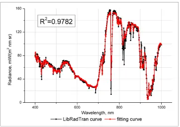
Figure 2. Spectral radiance on TOA according to LibRadTran calculations and fitting an analytic function (21)
radiation. What is this correspondence? A numerical calculation of the spectral radiance is carried out for a separate observation beam (as well as expression (17)), i.e. the problem is one-dimensional one. The surface and atmosphere are horizontally uniform, whereas the experimental value of the spectral radiance from satellite sensor is averaged over the finite instantaneous field of view corresponding to single pixel. In the numerical calculation of spectral radiance, the adjacency effect is not taken into account. It is also omitted in the analytical equations in this validation part (in Eq.17should be substitutedρeλ = ρλ), but it is taken into account for real satellite data (there is a problem of the neighborhood influence selection, that is select of the adjacency effect radius). Furthermore, in measured spectral radiance of hyperspectrometer ’s instrumental errors is present, due to its response function, inherent noise etc, which is not fully compensated by means of radiometric correction procedure. Whereas numerically calculated spectral radiance, such errors is determined by calculation.
(a)Water (b)Bare soil
(c)Grass (d)Snow
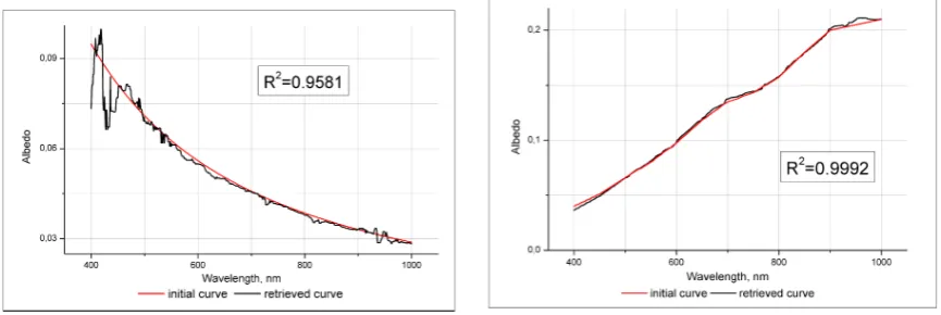
Figure 3.The albedo spectra for four different types (water3a, bare soil3b, grass3cand snow3d) retrieved by SHARC technique using the numerically calculated (LibRadTran) outgoing TOA radiance spectra, compared to the albedo spectra, initially given in direct problem.
As shown numerical calculations, the accuracy of the emission spectrum at the top of atmosphere by analytical equations is very high, which is confirmed by Fig.2, On Figure2shown two curves of the brightness (instead of the reflection coefficient) at TOA direct problem: obtained by numerical calculation of LibRadTran with the underlying surface "grass" and fitting curve of non-linear least squares LM algorithm with the analytical Eq(21).
(a)Image was acquired 17.04.2002 (sun elevation angle: 63.1 deg) and covers territory of south part of Arabian Peninsula (12.96433N 43.42845E)
(b)Image was acquired 23.08.2007 (sun elevation angle: 55.46 deg) and covers territory of California (Lake Tahoe, 38.86396N 120.01512W)
(c)Image was acquired 25.10.2014 (sun elevation angle: 34.78 deg) and covers territory near city of Haifa, Israel (32.82167N 35.09679E)
Figure 4. RGB–images of the Hyperion hyperspectrometer is based on retrieved spectral albedo functions by the SHARC method.
surfaces (water, soil, grass, snow) obtained by SHARC technique with using numerically calculated (LibRadTran) TOA brightness spectra, in comparison with the true albedo one given in the direct task (as input data for LibRadTran). The error in retrieves by the determination coefficientsR2is characterized, showed on each of figures. Figure3reflects the typical retrieved albedo profile errors obtained for other types of underlying surfaces.
In addition, atmospheric correction of hyperspectral satellite images obtained using the Hyperion sensor on the Earth Observer-1 (EO-1) was performed. Three different images with different types of surface were selected, including various types of underlying surfaces water, sand, green vegetation, rocks, etc., shown in Figure4.
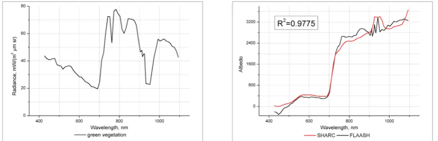
Results of the SHARC method were compared with atmospheric correction data of these images in the well-known FLAASH module, implemented in ENVI software package. Typical comparison results for images of Hyperion sensor are shown in Figs.5,6,7. In the left hand side of figures the pixel brightness spectra in absolute units (after radiometric correction) registered by the sensor are shown. The right hand side contains the albedo spectra retrieved by SHARC method and FLAASH module.
It should be noted that the retrieved profiles of the albedo SHARC and FLAASH are in satisfactory agreement. In this case, the SHARC curve is smoother in comparison with FLAASH and shows somewhat better (smoother) behavior in the region of the absorption bands of water vapor around 940nm. The good enough "smoothness" of the albedo spectral profiles reconstructed by the SHARC method in the absorption band of atmospheric gases (both in the calculated spectra of LibRadTran and in Hyperion satellite spectrum images) for the absorption in water vapor bands by two parametersm11 andm12, and calculated in advance of standard transmission is a consequence of good approximation in our case. In addition, FLAASH curve often gives negative albedo values at some spectral ranges (Figures6and7).
In some cases, the Hyperion sensor gives insufficient quality, as shown, in Fig.7for the water surface, where the original spectrum contains "emission bands" behind 900nm, which are either an artifact or correspond to the presence of an unusual component in the water spectrum.
Earth Observation Satellites [23]. This portal provides is open access bottom-of-atmosphere (BOA) and TOA reflectance data measured derived over a network of sites. The data continuously updated, have a 10 nm spectral sampling interval in the spectral range from 380nmto 2500nm.
The Hyperion image that covers of the La Crau site with location in the south of France (43.55N 4.85W) was found. This site area has a thin pebbly soil with sparse vegetation cover [24]. Figure8
shows the Hyperion image footprint (red rectangle) with location near La Crau (yellow mark). The Hyperion image was acquired 29.10.2016, UTC time 7:48:20 (sun elevation angle: 14.6 deg). RadCalNet data were measured 29.10.2016, UTC time 9:00 (sun elevation angle: 24.11 deg).
6. Conclusions
A new algorithm for atmospheric correction of hyperspectral images SHARC is presented. The algorithm enables the determination of the albedo of the underlying surface "on the fly" without using a priori information about the atmosphere and the surface. Also we do not use LUTs or time consuming numerical solutions of the radiative transfer equation. Instead the algorithm uses a parameterized analytical solution of the radiative transfer equation for TOA outgoing radiation for a wide range of atmospheric parameters, including practically all cloudless one. The type of atmospheric aerosol is not predetermined depending on the season and geographical location of the survey, but it is characterized by four unknown parameters accounting for almost all possible types of aerosols.
The advantage of the proposed method is a very short time of performing the procedure of atmospheric correction even for very large images (about a few seconds on a personal computer of standard configuration) with good accuracy of the albedo retrieving. The limitation of the method is the above-mentioned range of atmospheric parameters, for which approximations of the functions have been obtained:ga∈[0−0.9],τ∈[0−2],µ∈[0.2−1.0], which, however, covers most realizations of the cloudless atmosphere. Another limitation is the assumption of a horizontal homogeneity of the atmosphere within the image, since the parameters of the atmosphere are assumed to be the same for all pixels. If this assumption is not fulfilled (for example, for large images), the proposed correction method can be applied successively to image subsets (areas) to which the original image should be divided (for example, using a sliding rectangular window) and within which the independent parameters of the atmosphere are obtained. We plan to further develop the method, taking into account the possible horizontal inhomogeneity of the atmosphere, as well as the non-flat terrain.
References
1. Eismann M. Hyperspectral Remote Sensing. Editor, Press., 2012; pp. 725.
2. Miller C. J. Performance assessment of ACORN atmospheric correction algorithm.Algorithms and Technologies for Multispectral, Hyperspectral, and Ultraspectral Imagery VIII, SPIE2002,4725, 438-449.
3. Richter R.; Schlapfer D. Geo-atmospheric processing of airborne imaging spectrometry data. Part 2: Atmospheric/topographic correction.Int. J. of Remote Sensing2002,23, 2631-2649.
4. Gao B.-C.; Heidebrecht K. B.; Goetz A. F. H. Derivation of scaled surface reflectances from AVIRIS data.
Remote Sensing of Environment1993,44, 165-178.
5. Adler-Golden S. M.; Matthew M. W.; Bernstein L. S.; Levine R. Y.; Berk A.; Richtsmeier S. C.; Acharya P. K.; Anderson G. P.; Feldeb G.; Gardner J.; Hokeb M.; Jeong L. S.; Pukall B.; Mello J.; Ratkowski A.; Burke H.H. Atmospheric correction for short-wave spectral imagery based on MODTRAN4.Imaging Spectrometry V, Denver. CO. SPIE1999,3753, 61-69.
6. Goetz A. F. H.; Kindel B. C.; Ferri M.; Qu Z. HATCH: Results from simulated radiance, AVIRIS and Hyperion.
JIEEE Transactions on Geoscience and Remote Sensing2003,6(41), 1215-1222.
7. Qu Z.; Kindel B. C.; Goetz A. F. H. The high accuracy atmospheric correction for hyperspectral data (HATCH) model.IEEE Transactions on Geoscience and Remote Sensing2003,6(41), 1223-1231.
9. Leprieur C.; Carrere V.; Gu X. F. Atmospheric corrections and ground reflectance recovery for Airborne Visible/Infrared Imaging Spectrometer (AVIRIS) data: MAC Europe’91.Photogrammetric Engineering and Remote Sensing1995,61(10), 1233-1238.
10. Katsev I. L.; Prikhach A. S.; Zege E. P.; Grudo J. O.; Kokhanovsky A. A. Speeding up the aerosol optical thickness retrieval using analytical solutions of radiative transfer theory. Atmos. Meas. Tech. 2010, 3, 1403–1422.
11. Katkovskii L.V. Parametrizatsiya ukhodyashchego izlucheniya dlya bystroi atmosfernoi korrektsii giperspektral’nykh izobrazhenii (The parameterization of the outgoing radiation for rapid atmospheric correction of hyperspectral images).Optika atmosfery i okeana.2016,29(9), 778-784.
12. Bucholtz A. Rayleigh-scattering calculations for the terrestrial atmosphere. Applied Optics1995, 34(15), 2765-2773.
13. Ginzburg A.S.; Romanov S.V.; Fomin B.A. Ispol’zovanie radiatsionno-konvektivnoi modeli dlya otsenki temperaturnogo potentsiala parnikovykh gazov. (The radiation-convective model use to estimate the temperature of greenhouse gas potential).Izvestiya RAN. Fizika atmosfery i okeana.2008,44(3), 324-331. 14. Ginzburg A.S.; Mel’nikova I.N.; Samulenkov D.A.; Sapunov M.V.; Katkovskii L.V.; Prostaya. Prostaya
opticheskaya model’ bezoblachnoi i oblachnoi atmosfery dlya rascheta potokov solnechnoi radiatsii. (A simple optical model cloudless and cloudy atmosphere to calculate solar radiation fluxes.) Sovremennye problemy distantsionnogo zondirovaniya Zemli iz kosmosa.2016,13(2), 132–149.
15. Belyaev B.I.; Belyaev M. Yu.; Desinov L. V.; Katkovsky L.V.; Sarmin E. E. Obrabotka spektrov i izobrazhenii s fotospektral’noi sistemy v kosmicheskom eksperimente “Uragan” na MKS (Spectral and Images Processing from Photospectral System in Space Experiment "HURRICANE" on the ISS).Issledovanie zemli iz kosmosa.
2014,6, 54–65.
16. Vasil’ev A.V.; Kuznetsov A.D.; Mel’nikova. I.N. Distantsionnoe zondirovanie okruzhayushchei sredy iz kosmosa: praktikum. (Remote sensing of the environment from space: practice). Editor, Balt.State Tech.University, St.-Petersburg; 2008; pp. 33.
17. Minin I.N. Priblizhennye formuly dlya raschetov pogloshcheniya korotkovolnovogo izlucheniya v bezoblachnoi atmosfere (Approximate equations for short-wave radiation absorption calculations in cloudless atmosphere).Izv. AN SSSR. Fiz. atm. i okeana.1984,20(10), 999-1001.
18. Kokhanovsky A.A.; Mayer B.; Rozanov V.V. A parameterization of the diffuse transmittance and reflectance for aerosol remote sensing problems.Atmos. Research2005,73, 37–43.
19. Vasil’ev A.V.; Kuznetsov A.D.; Mel’nikova. I.N. Approksimatsiya mnogokratno rasseyannogo solnechnogo izlucheniya v ramkakh priblizheniya odnokratnogo rasseyaniya. (Approximation of multiply scattered solar radiation in the assumption of single scattering). International Symposium "Atmospheric Radiation and Dynamics" (ISARD 2015); Saint-Petersburg- Petrodvorets, 23 – 26 June 2015; 2015; pp. 131
20. Middleton, W. E. K. Vision through the Atmosphere, University of Toronto Press, Toronto, (1952).
21. Schlapfer D., Borel C. C., Keller J.,and Itten K. I. Atmospheric Precorrected Differential Absorption Technique to Retrieve Columnar Water Vapor.Remote Sensing of Environment1998,65, 353–366.
22. Bassani C., Cavalli R. M., and Antonelli P. Influence of aerosol and surface reflectance variability on hyperspectral observed radiance.Atmos. Meas. Tech.2012,5, 1193–1203.
23. https://www.radcalnet.org/
(a)Coastal Water; label#1 in Figure4a
(b)Green Vegetation; label#2 in Figure4a
(c)Sand; label#3 in Figure4a
(a)Green Vegetation; label#1 in Figure4b
(b)Rocks; label#2 in Figure4b
(c)Coastal Water; label#3 in Figure4b
(a)Soil; label#1 in Figure4c
(b)Green Vegetation; label#2 in Figure4c
(c)Water; label#3 in Figure4c
Figure 8. La Crau site with Hyperion image footprint.