Article
1
The role of synoptic cyclones for the formation of
2
Arctic summer circulation patterns as clustered by
3
self-organizing maps
4
Min-Hee Lee 1 and Joo-Hong Kim 1,*
5
1 Korea Polar Research Institute, 26, Songdomirae-ro, Yeonsu-gu, Incheon 21990, Korea; [email protected]
6
* Correspondence: [email protected]
7
8
Abstract: The contribution of extra-tropical synoptic cyclones to the formation of summer-mean
9
atmospheric circulation patterns in the Arctic is investigated by clustering the dominant Arctic
10
circulation patterns by the self-organizing maps (SOMs) using the daily mean sea level pressure
11
(MSLP) in the Arctic domain (≥ 60°N). Three SOM patterns are identified: one with prevalent low
12
pressure anomalies in the Arctic Circle (SOM1) and two opposite dipoles with primary high
13
pressure anomalies covering the Arctic Ocean (SOM2 and SOM3). The time series of summertime
14
occurrence frequencies demonstrate the largest inter-annual variation in the SOM1, the slight
15
decreasing trend in the SOM2, and the abrupt upswing after 2007 in the SOM3. The relevant
16
analyses with produced cyclone track data confirm that the vital contribution. The Arctic cyclone
17
activity is enhanced in the SOM1 because the meridional temperature gradient increases over the
18
land–Arctic Ocean boundaries co-located with major cyclone pathways. The composite daily
19
synoptic evolutions for each SOM reveal that the persistence of all the three SOMs is less than 5 days
20
on average. These evolutionary short-term weather patterns have substantial variability at
inter-21
annual and longer timescales. Therefore, the synoptic-scale activity is central to forming the
22
seasonal-mean climate of the Arctic.
23
Keywords: Arctic summer circulation patterns, Extra-tropical synoptic cyclones, Self-organizing
24
maps (SOMs), Cyclone detection and tracking
25
26
1. Introduction
27
Low-frequency atmospheric circulation modes in the Arctic (e.g., the Arctic Oscillation (AO),
28
Dipole Anomaly (DA), etc.) have been of high interest as a controlling factor of the spatio-temporal
29
sea-ice variability [1–3], as it could have been investigated in various methods through relatively
30
more abundant atmospheric data sources, compared with the ocean circulation pattern. Among
31
seasons, the summer circulation pattern has been paid attention as its temporal proximity to the
32
September sea-ice minimum [4–9]. However, earlier preconditioning factors during previous winter
33
and spring have been also attracted much attention due to their value for long-lead seasonal
34
prediction [10–12].
35
The summer season is known to be the most synoptically active in the Arctic Ocean [13–15]. As
36
high-latitude sea-ice and snow gradually disappear by seasonal warming, the meridional thermal
37
contrast between the land and ocean preferentially forms the baroclinic frontal zone along the
land-38
ocean boundary [16]. As a result, the summer in the Arctic Ocean is stormier than the winter, by local
39
cyclogenesis, as well as by migratory mid-latitude cyclones [14]. Therefore, the Arctic cyclone itself
40
and its role in controlling sea-ice have been critical topics to understand the Arctic summer [17–19].
41
In a scale interaction perspective, the Arctic is a singular region where the zonal scales from
42
synoptic to planetary merge, due to reduced length of latitudinal circles. If a strong synoptic
43
cyclone/anticyclone persists or synoptic cyclones/anticyclones frequently pass near the pole, it can
44
directly contribute to the low-frequency (i.e., monthly-to-seasonal) large-scale circulation pattern
45
therein [13,14,20]. [14] showed that the cyclone activity is dominant during the cyclonic summer sea
46
level pressure pattern through the composite analysis and case investigation. On the other hand, [20]
47
revealed that the episodic synoptic anticyclones in the Arctic favor anticyclonic summer seasonal
48
circulation that accounts for more summer sea-ice melting.
49
As described above, previous studies suggested that the accumulation of synoptic events is
50
relevant for generating a preferred pattern of seasonal circulation in the Arctic, but none of them tried
51
to investigate the quantitative contribution of synoptic cyclones to individual summer-mean
large-52
scale circulation patterns in the Arctic. Accordingly, the detection and tracking of extra-tropical
53
synoptic cyclones are carried out to quantify cyclone activity and relate it with the summer-mean
54
Arctic circulation patterns. We also need to identify the summer-mean Arctic circulation patterns
55
with a relevant pattern classification method. Among methods, we adopt the self-organizing maps
56
(SOMs) which has been proven to effectively distinguish the representative patterns from the large
57
climate data set [21–24]). [21] have identified the continuum of El Niño–Southern Oscillation
(ENSO)-58
related sea surface patterns. [22] have used for distinguishing the shift of atmospheric jet that are not
59
separated by empirical orthogonal functions (EOFs). In addition, the SOMs have been used to
60
distinguish the patterns related to the variabilities of the winter cold extremes over North America
61
and Europe [23] and the summer hot extremes over the Northern Hemisphere [24]. These studies
62
have concluded that the clusters derived from the SOMs are more accurate and linearly independent
63
than those from commonly used hierarchical cluster analysis.
64
This study is structured as follows. Section 2 provides the descriptions of the data and analysis
65
methods including the SOM clustering, detection and tracking of synoptic cyclones and grid-cell
66
representation of cyclone activity. Section 3 presents the representative SOM patterns of Arctic
large-67
scale surface circulation during summer and their inter-annual variations. Furthermore, associated
68
with individual SOM patterns, this section also shows the synoptic cyclone activities, the analyses
69
relevant to the cyclone development and the daily synoptic evolution of large-scale circulation in the
70
Arctic. Finally, summary and discussions are given in Section 4.
71
2. Data and Methods
72
2.1. Data
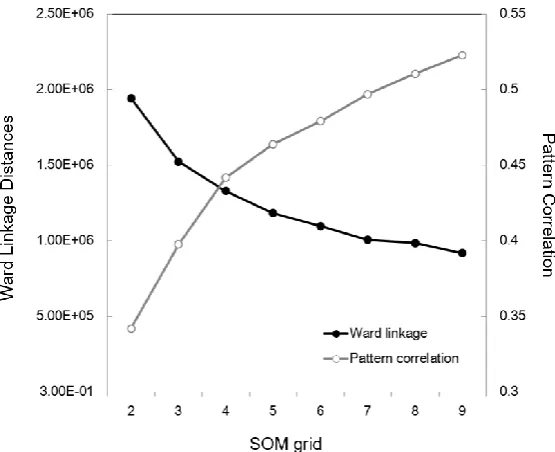
73
This study primarily used the atmospheric fields of the European Centre for Medium-Range
74
Weather Forecasts Interim Reanalysis (ERA-Interim) dataset [25] with the 1.5°
1.5° horizontal75
resolution during boreal summer (June-July-August, JJA) of 1979–2017. The SOM clustering
76
algorithm utilized the daily mean sea level pressure (MSLP) field with its climatological-mean of
1-77
2-1 smoothed daily seasonal cycle being removed. The further atmospheric analyses corresponding
78
to SOM clusters were carried out with the horizontal winds, temperatures, and geopotential heights
79
between 850 hPa and 200 hPa. For storm detection, the 6-hourly fields of the MSLP and 850-hPa
80
relative vorticity were used as the input for the storm detection algorithm used (see Section 2.3).
81
2.2. Self-organizing maps (SOMs)
82
The SOM algorithm is one of the clustering methods, which originates form neural networks
83
(refer to the appendix in [26] for more details). Because it is based on the K-means clustering, it
84
classifies data into a specified number of clusters through supervised machine learning. It differs
85
from the other clustering methods in that it relocates the resultant clustering patterns onto a one- or
86
two-dimensional grid based on the pattern similarity between clusters [27]. This ad-hoc relocation
87
enables us to describe a continuum of atmospheric circulation regimes [21,26,28].
88
During the training period, individual data are partitioned into a particular SOM pattern to
89
which the Euclidean distance from the data is minimum. Here it means that each daily MSLP pattern
90
should have its best-matching SOM pattern. Naturally the two patterns match better as the
91
predefined number of SOM patterns increases, but too large numbers of SOM clusters are less useful
92
for clearly identifying the different physical modes in the data. Therefore, it is generally
recommended to determine the optimal number of SOM patterns by satisfying the following two
94
conditions; (1) the number of SOM patterns is large enough to accurately capture the physical
95
characteristics of the data, and, at the same time, (2) it needs to be sufficiently small so that the clusters
96
are distinctive from each other. To find the optimal number of SOM patterns satisfying the both
97
conditions, we compute (1) the average pattern correlations between the daily fields and their
best-98
matching SOM pattern [22] and (2) the distance between different cluster pairs (d: Ward’s linkage
99
distance) using the following definition as in [24]:
100
101
𝑑(𝑟, 𝑠) = √2𝑛𝑟𝑛𝑠
(𝑛𝑟+𝑛𝑠)‖𝑥̅𝑟− 𝑥̅𝑠‖2 (1)
102
where nr and ns are the number of elements in clusters r and s, respectively, and 𝑥̅𝑟 and 𝑥̅𝑠 are the
103
centroid patterns of clusters r and s, respectively. The equation was obtained from the concept of
104
Ward’s linkage, which computes the merging cost of two clusters in a hierarchical cluster method.
105
According to previous studies [24,29], this concept can be applied to measure the distinctiveness
106
between clusters.
107
108
Figure 1. Ward linkage distances between SOM patterns (open circle, left y-axis), and average pattern
109
correlations of the daily MSLP fields with their best-matching SOM pattern (closed circle, right y-axis) as a
110
function of a single-column SOM grid.
111
2.3. Cyclone tracking and gridding
112
For detection and tracking extra-tropical cyclones, the method of [30] is used without the criteria
113
for tropical cyclone detection. Detecting cyclone centers in the Northern Hemisphere extra-tropics
114
(north of 30°N) comprises the following three criteria: 1) a local maximum of the 850-hPa relative
115
vorticity larger than 2.0×10⁻⁵ s-1 within each 11×11 grid window, 2) the closest local minimum of the
116
MSLP within a 400 km radius of the local vorticity maximum found from 1), and 3) the MSLP increase
117
by at least 15 Pa in all directions within a 500 km distance from the local pressure minimum found
118
by 2). Followed by detecting all cyclone centers, the tracking procedure creates the temporal
119
movement of the detected cyclones by the technique to determine the most probable migrated
120
position at the next time step. The procedure has three steps as follows: 1) Detected cyclone centers
121
are picked up within the circular tracking boundary (radius: 750 km) from a cyclone center at the
122
previous time step. 2) In case of picking up one center within the boundary, it is taken as the migrated
123
cyclone position. If there exist multiple centers, the algorithm gives priority to the nearest center in
124
the front semicircle towards the moving direction of the cyclone, but if not, the nearest one regardless
125
of the direction is chosen. If no cyclones are detected within the boundary, the algorithm stops
tracking that cyclone. 3) Among the output data of cyclone tracks, those with lifetime shorter than
127
1.5 days are discarded. Then the remaining cyclone tracks are archived to the final cyclone track
128
database.
129
Transforming cyclone tracks into grid-cell counts has a merit for clearly presenting the
130
distribution of cyclone activity [31]. Due to a singularity near the pole, we construct equidistant
grid-131
cells with 500 km by 500 km centering on the pole, rather than conventional latitude-longitude
grid-132
cells. The gridded spatial distribution is constructed for each summer. Then the gridded data are used
133
for yielding climatology or composite. In this study, the grid-cell cyclone frequency is shown for the
134
spatial distribution of cyclone activity, which is defined by counting only once when a cyclone enters
135
that grid
136
3. Results
137
3.1. SOM patterns of the summer MSLP in the Arctic
138
The SOM analysis is applied to the daily summer MSLP fields over the Arctic domain (north of
139
60°N) for the period of 1979-2017. Repeated SOM analyses are carried out with varying SOM grids
140
from (21) to (101). As described in Section 2.2, the optimal number of SOM clusters need to be
141
objectively determined, because distinctive atmospheric circulation patterns are the bases for
142
comparing the features of cyclone activity among the patterns. Here we follow the selection method
143
by Lee et al. (2017). As the number of SOM patterns increases, the mean pattern correlations (grey
144
line) increase, while the Ward’s linkage distances (black line) decrease (Figure 1). The significant test
145
with Monte Carlo random resampling reveals that the mean pattern correlations for all SOM grids
146
are statistically significant at the 5% level. However, the decreasing tendency of Ward’s linkage
147
distances is appreciably slower when the SOM number increases from (31) to (41). This is an
148
indication that the (31) grid can be the lowest optimal number enough to yield distinct SOM patterns
149
[24]. We therefore select the (31) grid as the appropriate number of SOM patterns classifying the
150
summer atmospheric circulation in the Arctic.
151
152
153
Figure 2. The SOM patterns of MSLP anomalies (hPa, top) and their time series of seasonal frequency of
154
occurrences (day number, bottom) per summer. The percentage for each SOM indicates the occurrence
155
frequency of that SOM pattern for 3588 days of boreal summers during 1979–-2017. The dotted lines
156
delineate the selected core areas for yielding the cyclone activity indices used in Table 2 (SOM1: positive
157
core ≥ 1 hPa, negative core ≤ −2 hPa, SOM2: positive core ≥ 2 hPa, negative core ≤ −2 hPa, SOM3: positive
158
core ≥ 2 hPa, negative core ≤ −1 hPa).
159
160
Figure 2 shows spatial patterns of three SOMs (SOM1, SOM2 and SOM3) and time series of their
161
individual occurrence frequencies for each summer (i.e., JJA). The frequency of occurrence was
obtained by counting the number of days showing the best match with a particular SOM pattern. It
163
is found that the three SOMs almost evenly divide the summer days, indicative of three major
164
patterns in the Arctic summer MSLP. The SOM1 shows that the negative MSLP anomaly prevails
165
over the Arctic Ocean, except over the northern Europe, and its frequency of occurrence largely
166
fluctuates year-to-year for the whole period (Figure 2a). The pattern resembles the polar branch of
167
the AO during its positive phase [2, 5].
168
Next the SOM2 represents the dipole anomaly (DA) between the Atlantic Arctic sector and the
169
Eurasian Arctic–Canada Basin sector (Figure 2b). Although this summertime DA of the SOM2 has a
170
node slightly rotated counterclockwise, compared with the summertime DA of Figure 2d in [3]
171
derived from the empirical orthogonal function (EOF) analysis, it is reasonable to say that our SOM2
172
DA is qualitatively similar to the negative phase of the DA of [3]. Compared with the other SOM
173
patterns, the SOM2 has relatively lower inter-annual variability, as well as a slight decreasing trend.
174
By contrast, the SOM3 appears a DA-like pattern which takes on a shape opposite to the SOM2,
175
but the node of the DA exists along the Eurasian Arctic seas (Figure 2c). It is qualitatively similar to
176
the positive phase of the DA of [3] related with the reduction of Arctic sea-ice, which represents the
177
anomalous anticyclonic pattern prevailing over the Canada Basin [6,9,20]. Interestingly, an abrupt
178
increase since 2007 has been shown in the time series of the SOM3 occurrence frequency, when a large
179
decreasing jump occurred in the time series of Arctic sea-ice extent.
180
The SOM-based clustered patterns in the Arctic MSLP have both similarities and discrepancies
181
in the shape, compared with the previous EOF-based circulation patterns. The SOM analysis has
182
advantages over the EOF analysis, in terms of its capability to yield asymmetric features and extract
183
complex patterns [32]. Thus it is thought that the three SOM patterns reflect the real climate regimes
184
in the summer surface atmospheric circulation of the Arctic.
185
3.2. Cyclone activities associated with the SOMs
186
Based on the three Artic surface circulation regimes (SOM1–3), here we try to identify the role
187
of synoptic cyclone activity in forming individual circulation regimes. First, the composite maps of
188
grid-cell cyclone frequency are constructed for the top five years with the high occurrence frequencies
189
of individual SOMs. It is noted that the selection of years for composite uses the detrended time series.
190
Table 1 lists the selected five years for each SOM pattern. The chosen five years for composite
191
correspond to the top 12.5th percentile during the 39 years of 1979–2017. The results are insensitive
192
to the number of chose years from the top four (10th percentile) to six (15th percentile) years (not
193
shown).
194
195
Table 1. The top five years used for composite selected from the detrended time series of occurrence
196
frequencies for each SOM.
197
198
SOM Top five years
1 2006, 1983, 2017, 1994, 1989 2 1979, 1990. 1985, 2004, 2013 3 2015, 1980, 2007, 2011, 2009
199
Figure 3 presents the resultant climatological distribution of extra-tropical cyclones for the
200
period of 1979–2017 (3a) and the composite anomalies associated with the top five years of individual
201
SOMs (3b–d). According to [14], summer cyclones in the Arctic can be developed within the Arctic,
202
due to enhanced thermal contrast between land and the Arctic Ocean. Consistent with their study,
203
the activity core over the Arctic Ocean is obvious, in addition to two mid-latitude cores in the North
204
Pacific and North Atlantic Oceans (Figure 3a).
205
The composite anomalies of grid-cell cyclone frequencies in the SOM1 high years show a
206
remarkable increase over the central Arctic Ocean and Greenland–Norwegian seas (Figure 3a).
207
Meanwhile, the cyclone frequencies in the mid-latitude North Atlantic and the Bering Sea, which are
208
the regions where cyclone activity is climatologically frequent, tend to decrease in the SOM1 high
years. Considering the distribution of cyclone frequencies, the seasonal formation of the SOM1
210
pattern is closely linked to the higher synoptic cyclone activity over the central Arctic Ocean and
211
Greenland–Norwegian seas. The MSLP anomalies associated with the SOM2 pattern are
212
characterized by the dipole pattern between the Eurasian Arctic–Canada Basin sector and the Atlantic
213
Arctic sector (Figure 2b). Consistent with the circulation pattern, the composite anomalies of grid-cell
214
cyclone frequencies also show the dipole with positive anomalies around Greenland and the
215
Canadian Arctic Archipelago and negative anomalies in the Eurasian Arctic side during the SOM2
216
high years (Figure 3c). During the SOM3 high years, the overall cyclone frequencies over the Arctic
217
Ocean are significantly reduced (Figure 3d). Meanwhile, the cyclone frequencies in the mid-latitude
218
North Atlantic and the Bering Sea increase, but those cyclones seem to seldom migrate into the Arctic
219
Ocean. As the SOM3 pattern is the dipole dominated by the high pressure in the Arctic Ocean area
220
(Figure 2c), it matches well with the SOM3 composite anomalies of grid-cell cyclone frequencies.
221
222
223
Figure 3. Climatological map of cyclone frequencies (# year−1) for the period 1979–2017 (a) and their
224
composite anomalies for the top five years selected from the detrended time series of occurrence frequencies
225
for each SOM (b–d). The dots denote the grids where the anomaly is statistically significant at the 10% level
226
by the Monte Carlo test.
227
228
The comparison of spatial patterns (Figure 2 vs. Figure 3) qualitatively displays the relevance of
229
synoptic cyclone activity to the formation of summer-mean circulation patterns in the Arctic. For
230
statistically quantifying the contribution of cyclones over the entire analysis period, the temporal
231
correlation analysis is performed using the time series of cyclone activity indices (i.e., frequency,
232
duration, and mean intensity) and summer-mean MSLP. The positive and negative core areas of
233
individual SOMs are selected for constructing the time series, which are based on the anomaly
patterns in Figure 2. The frequency is constructed by counting the number of cyclones passing the
235
core area, while the duration multiply counts all 6-hourly cyclone positions for all cyclones within
236
the core area, then dividing the number by 4 to express in units of days. The mean intensity is defined
237
as the average of 6-hourly central pressure data for all 6-houly cyclone positions within the core area.
238
239
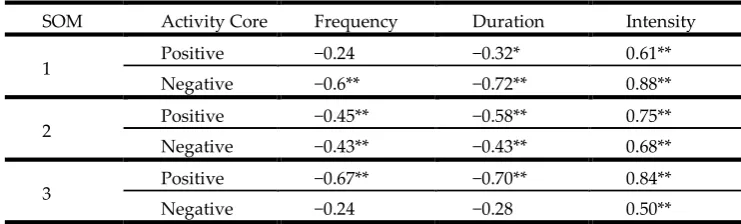
Table 2. Correlation coefficients of the time series of summer-mean MSLP anomalies with three cyclone
240
activity indices (i.e., frequency, duration and mean intensity) for the positive and negative core areas of each
241
SOM (dotted lines in Figure 2). All the time series are obtained by averaging within individual core area.
242
The significant correlations are denoted by one (p-value: 0.05) and two asterisks (p-value: 0.01) by the
two-243
sided Student’s t test.
244
245
SOM Activity Core Frequency Duration Intensity
1 Positive −0.24 −0.32* 0.61**
Negative −0.6** −0.72** 0.88**
2 Positive −0.45** −0.58** 0.75**
Negative −0.43** −0.43** 0.68**
3 Positive −0.67** −0.70** 0.84**
Negative −0.24 −0.28 0.50**
246
247
The resultant correlation coefficients reveal that, among the indices, the mean intensity has the
248
highest absolute correlations that are statistically significant at 5% level for all core areas of all SOM
249
patterns (Table 2). This result stands to reason because the cyclone central pressure itself is the
250
variable equivalent to the MSLP. Therefore the overall cyclone intensity is the most effective
251
determiner of the seasonal-mean MSLP anomaly pattern in the Arctic. The duration is the second
252
effective determiner and the frequency is the last, though in some cases (e.g., the negative core area
253
of the SOM2, the positive core area of the SOM3) the frequency plays a significant role that is almost
254
equivalent to the duration. Over the positive core area of the SOM1 and the negative core area of the
255
SOM3, neither the frequency nor the duration of synoptic cyclones are effective indices for the
256
formation of the seasonal-mean MSLP anomaly. However, these areas are not primary cores, but
257
secondary in those SOM patterns (Figure 2).
258
3.3. Large-scale fields relevant to the cyclone activity forming each SOM
259
We have shown that the spatio-temporal variation of extra-tropical cyclones contributes
260
significantly to the formation of the summer-mean circulation pattern in the Arctic. Now it is
261
necessary to understand the large-scale atmospheric fields providing a background for their
spatio-262
temporal variation. As a primary energy source of extra-tropical cyclones, the baroclinic instability is
263
modulated by the changes in the meridional temperature gradient (the vertical shear of horizontal
264
winds), thus we display the composite anomalies of the 200-hPa zonal wind (U200) and skin
265
temperature (Ts) for the top five years of individual SOMs (Figure 4). As an indicator of baroclinicity,
266
the Eady growth rate and the vertical shear of zonal winds (200 minus 850 hPa) were also
267
investigated, but the U200 is solely shown as it primarily determines both the Eady growth rate and
268
the vertical wind shear. In the climatological pattern, the summer Ts around the Arctic Circle shows
269
a large gradient between land and ocean, and the higher speed of U200 appears along the
mid-270
latitude jets (Figure 4a).
271
For the SOM1 high years (Figure 4a), warm Ts anomalies are distributed over the Western
272
Europe, Ural Mountains, Northern Territories of Canada, and far-eastern Russia, while weaker cold
273
Ts anomalies are located north of those warm Ts anomalies. This indicates the stronger meridional
274
temperature gradient and thus forms the positive U200 anomalies (i.e., the larger vertical shear of
275
zonal winds) north of the warm Ts anomalies. The faster U200 prevails over the Arctic Ocean rim and
276
the northern North Atlantic Ocean, leading to more frequent poleward migration of synoptic
cyclones from the North Atlantic Ocean as well as local cyclogenesis in the Arctic. Actually, this result
278
for the SOM1 high years can be naturally expected because the areas of the faster U200 coincide with
279
those with climatologically frequent cyclone activity such as the northern Russian coast, Canadian
280
Arctic Archipelago, and northern North Atlantic Ocean (Figure 3a).
281
Next, for the SOM2 high years (Figure 4b), there are two Arctic areas with warm Ts anomalies:
282
one from the Barents Sea towards the Taymyr Peninsula in the far north of Russia and the other over
283
Alaska, and also two Arctic areas with cold Ts anomalies: one over northeastern Russia and the other
284
over the Canadian Arctic Archipelago. However, the anomalies are only statistically significant over
285
the Barents Sea and northeastern Russia. Accordingly, the statistically significant U200 anomalies are
286
also appreciable around those regions. Though not as clear as for the composite anomalies in the
287
SOM1 high years, these overall U200 weakening surrounding the Eurasian Arctic could contribute to
288
the less cyclone activity therein (Figure 3c).
289
290
Figure 4. Same as Figure 3 except for the fields of Ts (shading, °C) and U200 (contour, m s−1). The dots and
291
hatches respectively denote the grids of Ts and U200 where their anomalies are significant at the 5% level
292
by the two-sided Student’s t test.
293
294
Lastly, composite anomalies in the SOM3 high years partly show a state opposite to those in the
295
SOM1 high years (Figure 4c). This means the reduced meridional temperature gradient and slower
296
U200 surrounding the Arctic Ocean rim and the northern North Atlantic Ocean, resulting in less
297
cyclone migration from the North Atlantic Ocean as well as overall reduced cyclogenesis in the Arctic
298
(Figure 3d).
299
3.4. Synoptic evolution associated with the SOMs
Given the significant role of synoptic cyclones in the formation of summer-mean Arctic
301
circulation patterns as clustered by the SOMs, it would be informative to characterize the generalized
302
daily evolution of synoptic activity for each SOM by constructing lead-lag composites based on the
303
central days (i.e., lag day 0) of each SOM. The central days of a certain SOM are the best-matching
304
days with the SOM pattern (Figure 2). Here consecutive days with the same SOM pattern is defined
305
as a single event of that SOM. If there are two or more days of one SOM event, the best-matching day
306
is selected among the days that has the smallest root mean square error (RMSE) between the daily
307
MSLP anomaly pattern and the SOM pattern. Through this searching process, we identify 109 events
308
of the SOM1, 112 of the SOM2, and 114 of the SOM3, respectively, for the period of 1979–2017. Prior
309
to constructing lead-lag composites, 15-day moving averages are subtracted from the daily data in
310
order to focus only on the synoptic-scale variability. In Figures 5–7, the daily evolutions for individual
311
SOMs are shown with the 500-hPa geopotential height (H500).
312
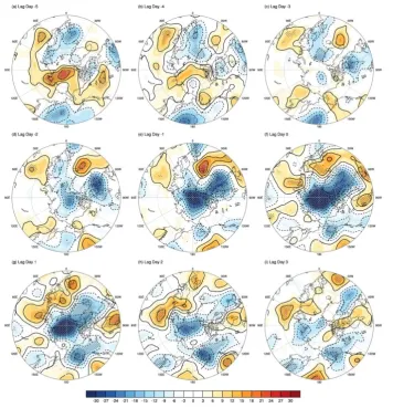
313
314
Figure 5. Composite daily evolutions of the synoptic-scale H500 anomalies (gpm) from −5 to +3 days for the
315
109 best-matching events of the SOM1. The dots denotes the grids where the anomalies are statistically
316
significant at the 5% level by the two-sided Student’s t-test.
317
318
The composite daily evolution associated with the 109 SOM1 events (Figure 5) shows as to how
319
the prevailing low pressure system takes up the entire Arctic Ocean at lag day 0 (Figure 5f). From lag
320
day −5 to −2 (Figure 5a–c), the northward migrating low pressure composite is detected in the
321
Norwegian Sea and the East Siberian Sea, where only the former is statistically significant at the 5%
322
level. They quickly erase the preexisting high pressure composite in the Central Arctic Ocean and get
323
stronger until lag day 0. Meanwhile, another low pressure composite develops around Quebec,
324
Canada and extends northward. Eventually a massive low pressure composite occupies the Arctic
Ocean towards Greenland (Figure 5f). The low pressure composite in the Arctic Ocean is sustained
326
significantly until lag day 2 (Figure 5h) and then weakens at lag day 3 (Figure 5i).
327
Figure 6 shows the composite daily evolution for the 112 best-matching events of the SOM2. At
328
lag day −5, a reversed dipole analogous to the SOM3 pattern exists (Figure 6a). This pattern is quickly
329
transformed to the incipient stage of the SOM2 during lag day −4 to −3 by the developing high
330
pressure composite over the Taymyr Peninsula and Laptev Sea and the developing low pressure
331
composite in-and-around Greenland (Figure 6b–c). These two opposite pressure systems further
332
develop and then the SOM2-like dipole pattern prevails in the Arctic from lag day −2 to lag day 1
333
(Figure 6d–g). After the SOM2 event, the low pressure system tends to prevail over the Arctic Ocean
334
(Figure 6h–i). Based on the composite evolutions, the SOM2 event seems to last shorter than the SOM1
335
event.
336
337
338
Figure 6. Same as Figure 5 except for the 112 best-matching events of the SOM2.
339
340
Lastly, the composite daily evolution is presented in Figure 7 for the 114 best-matching events
341
of the SOM3. Similar to the SOM2, there exist a dipole opposite to the SOM3 pattern at lag day −5
342
(Figure 7a). The high pressure composite around the Barents–Kara seas are pronounced, but it
343
weakens in three days (Figure 7b–d). The low pressure composite gradually develops and replaces
344
the high in the far north of Russia around the Kara–Laptev seas (Figure 7d–f), while the high pressure
345
composite begins to develop in the Beaufort Sea and then expands towards the central Arctic Ocean
346
(Figure 7b–f). The SOM3 event shows persistence after the peak day until lag day 3 (Figure 7g–i).
349
Figure 7. Same as Figure 5 except for the 114 best-matching events of the SOM3.
350
4. Summary and Discussion
351
The formation of monthly-to-seasonal atmospheric circulation patterns by low-frequency modes
352
in the Arctic has been extensively studied in terms of their influences on Arctic climate and sea ice
353
[1–9]. Researches have also shown that the activity of synoptic cyclones is more prevalent during
354
summer in the Arctic Ocean [13–15] and suggested their potential contribution to seasonal-mean
355
Arctic climate [13,14,20]. Our results further added the quantitative contribution of synoptic cyclone
356
activity to the amplitude of the seasonal-mean anomalies in the individual activity cores of three
357
dominant Arctic summer circulation patterns as clustered by the SOM method (Table 1), and also
358
confirm that the spatio-temporal distribution of synoptic cyclones in the Arctic domain is a major
359
controlling factor for the Arctic summer circulation patterns (Figures 2–3). Furthermore, the summer
360
cyclone activity in the central Arctic Ocean is enhanced only for the circulation pattern (e.g., SOM1)
361
that the land–Arctic Ocean boundary area with enhanced baroclinicity (i.e., the increased meridional
362
temperature gradient) is co-located with the climatological major cyclone pathways (Figures 3–4).
363
The composite daily synoptic evolutions well demonstrated the generalized formation processes
364
and the timescales of the three SOM patterns of the atmospheric circulation in the Arctic (Figures 5–
365
7). Although their evolutions have been shown with the high-pass filtered data by retaining only the
366
synoptic-scale variability, it is naturally expected to be almost consistent with those obtained from
367
the unfiltered daily data. The reason for this expectation is because the evolutionary SOM patterns as
368
shown in Figures 5–7 have just a couple of days timescale (i.e., within the synoptic-scale variability),
369
with e-folding times of 4.4, 3.6 and 3.6 days for the SOM1–3, respectively. According to previous
370
literature, these short timescale weather evolutions have substantial variability at inter-annual and
371
longer timescales beyond the climate noise [32– 34]. Therefore, it is reasonable to contend that the
summer-mean Arctic circulation patterns reflect the accumulation of short timescale events, such as
373
synoptic cyclones here or anticyclones as studied by [20].
374
The Arctic is not an isolated region but retains the Norther Hemispheric high-latitude
375
components of the global climate system that actively interact with lower latitudes [36–38]. Therefore,
376
the inter-annual and longer-timescale changes in the Arctic circulation patterns should be understood
377
in the context of global climate variability. Further studies are necessary to investigate as to which
378
type of climate variability over the globe provides a relevant teleconnection for the different summer
379
climatic states in the Arctic.
380
381
Author Contributions: Individual authors contributions are summarized as follows: “conceptualization, J.-H.K.;
382
methodology, M.-H.L.; formal analysis, M.-H.L.; writing—original draft preparation, M.-H.L. and J.-H.K.;
383
writing—review and editing, J.-H.K.; visualization, M.-H.L.; supervision, J.-H.K.; project administration, J.-H.K.;
384
funding acquisition, J.-H.K.”
385
Funding: This study was funded by the Korea Polar Research Institute (KOPRI) project, entitled ‘Development
386
and Application of the Korea Polar Prediction System (KPOPS) for Climate Change and Weather Disasters’
387
(KOPRI, PE19130).
388
Acknowledgments:
389
Conflicts of Interest: The authors declare no conflict of interest
390
References
391
1. Rigor, I.G.; Wallace, J.M.; Colony, R.L. Response of sea-ice to the Arctic Oscillation. J. Clim. 2002, 15, 2648–
392
2663, doi: 10.1175/1520-0442(2002)015<2648:ROSITT>2.0.CO;2.
393
2. Rigor, I.G.; Wallace J.M. Variations in the age of Arctic sea-ice and summer sea-ice extent, Geophys. Res. Lett.
394
2004, 31, L09401, doi: 10.1029/2004GL019492.
395
3. Wang, J.; Zhang, J.; Watanabe, E., Ikeda, M.; Mizobata, K.; Walsh, J.E.; Bai X.; Wu B. Is the Dipole Anomaly
396
a major driver to record lows in Arctic Summer sea ice extent? Geophys. Res. Lett. 2009, 35, L05706, doi:
397
10.1029/2008GL036706.
398
4. Ogi, M.; Wallace, J.M. Summer minimum Arctic sea ice extent and the associated summer atmospheric
399
circulation. Geophys. Res. Lett. 2007, 109, D20114, doi: 10.1029/2004JD004514.
400
5. Ogi, M.; Yamazaki, K. Trends in the summer northern annular mode and Arctic sea ice. SOLA 2010, 6, 41–
401
44, doi: 10.2151/sola.2010-011.
402
6. Ogi, M.; Wallace, J.M. The role of summer surface wind anomalies in the summer Arctic sea ice extent in
403
2010 and 2011. Geophys. Res. Lett. 2012, 39, L09704, doi: 10.1029/2012GL051330.
404
7. Screen, J.A.; Simmonds, I.; Keay, K. Dramatic interannual changes of perennial Arctic sea ice linked to
405
abnormal summer storm activity. J. Geophys. Res. 2011, 116, D15105, doi: 10.1029/2011JD015847.
406
8. Knudsen, E. M.; Orsolini Y.J.; Furevik, T.; Hodges K.I. Observed anomalous atmospheric patterns in
407
summers of unusual Arctic sea ice melt. J. Geophys. Res. 2015, 120, 2595–2611, doi: 10.1002/2014JD022608.
408
9. Ding, Q.; Co-authors. Influence of high-latitude atmospheric circulation changes on summertime Arctic sea
409
ice. Nat. Clim. Chang. 2017, 7, 289–295, doi: 10.1038/nclimate3241.
410
10. Kapsch, M.; Graversen R.G.; Tjernström M. Springtime atmospheric energy transport and the control of
411
Arctic summer sea–ice extent. Nat. Clim. Chang. 2013, 3, 744–748, doi: 10.1038/nclimate1884.
412
11. Park, H.-S.; Lee, S.; Kosaka, Y.; Son, S.-W.; Kim, S.-W. The impact of Arctic winter infrared radiation on
413
early summer sea ice. J. Clim. 2015, 28, 6281–6296, doi: 0.1175/JCLI-D-14-00773.1.
414
12. Williams, J.; Tremblay, B.; Newton, R.; Allard, R. Dynamic preconditioning of the minimum September
415
sea-ice extent. J. Clim. 2016, 29, 5879–5891, doi: 10.1175/JCLI-D-15-0515.1.
416
13. Zhang X; Walsh, J. E.; Zhang, J.; Bhatt, U.S.; Ikeda, M. Climatology and interannual variability of Arctic
417
cyclone activity: 1948–2002. J. Clim. 2004, 17, 2300–2317, doi:
10.1175/1520-418
0442(2004)017<2300:CAIVOA>2.0CO;2.
419
14. Serreze. M.C.; Barrett. A.P. The summer cyclone maximum over the central Arctic Ocean. J. Clim. 2008, 21,
420
1048–1065, doi: 10.1175/2007JCLI1810.1.
15. Orsolini, Y.J.; Sorteberg, A. Projected changes in Eurasian and Arctic summer cyclones under global
422
warming in the Bergen Climate Model. Atmos. Oceanic Sci. Lett. 2009, 2, 62–67, doi:
423
10.1080/16742834.2009.11446776.
424
16. Crawford, A.D.; Serreze, M.C. A new look at the summer Arctic frontal zone. J. Clim. 2015, 28, 737–754, doi:
425
10.1175/JCLI-D-14-00447.1.
426
17. Mesquita, M.; Kvamstø, N.G.; Sorteberg, A.; Atkinson, D.E. Climatological properties of summertime
extra-427
tropical storm track in the Northern Hemisphere. Tellus A. 2008, 60, 557–569, doi:
10.1111/j.1600-428
0820.2008.00305.x.
429
18. Simmonds, I. Rudeva, I. The great Arctic cyclone of August 2012. Geophys. Res. Lett. 2012, 39, L23709, doi:
430
10.1029/2012GL054259.
431
19. Semenov, A.; Zhang, X.; Rinke, A.; Dorn, W.; Dethloff, K. Arctic intense summer storms and their impacts
432
on sea ice – a regional climate modeling study. Atmos. 2019, 10, 218, doi: 10.3390/atmos10040218.
433
20. Wernli, H.; Papritz, L. Role of polar anticyclones and mid-latitude cyclones for Arctic summertime sea-ice
434
melting. Nat. Geosci. 2018, 11, 108–113, doi: 10.1038s41561-017-0041-0.
435
21. Johnson, N.C. How many ENSO flavors can we distinguish? J. Clim. 2013, 26, 4816–4827, doi:
436
10.1175/JCLI0D012099649.1.
437
22. Lee, S.; Feldstein, S.B. Detecting ozone- and greenhouse gas-driven wind trends with observational data.
438
Science 2013, 339, 563–567, doi: 10.1126/sciences.1225154.
439
23. Bao, M.; Wallace, J.M. Cluster analysis of Northern Hemisphere wintertime 500-hPa flow regimes during
440
1920–2014. J. Atmos. Sci. 2015, 72, 3597–3608, doi: 10.1175/JAS-D-15-0001.1.
441
24. Lee, M.-H.; Lee, S.; Song, H.-J.; Ho, C.-H. The recent increase in the occurrence of a boreal summer
442
teleconnection and its relationship with temperature extremes. J. Clim. 2017, 30, 7493–7504, doi:
443
10.1175/JCLI-D-16-0094.1.
444
25. Dee, D.P.; Co-authors. The ERA-Interim reanalysis: Configuration and performance of the data assimilation
445
system. Quart. J. Roy. Meteor. Soc. 2011, 137, 553–597, doi: 10.1002/qj.828.
446
26. Johnson. N.C; Feldstein, S.B.; Tremblay, B. The continuum of Northern Hemisphere teleconnection patterns
447
and a description of the NAO shift with the use of self-organizing maps. J. Clim. 2008, 21, 6354–6371, doi:
448
10.1175/20089JCLI2380.1.
449
27. Kohonen, T. Self-Organizng Maps, 3rd ed.; Springer 2001; 521pp.
450
28. Leloup, J.; Lachkar, Z.; Boulaner, J.-P.; Thiria, S. Detecting decadal changes in ENSO using neural networks.
451
Clim. Dyn. 2007, 28, 147–162, doi: 10.1007/s00382-006-0173-1.
452
29. Xu, G.; Zong, Y.; Yang, Z. Applied Data Mining.; CRC Press 2013; 284pp.
453
30. Vitart, F.; Anderson, J.L.; Stern, W.F. Simulation of interannual variability of tropical storm frequency in an
454
ensemble of GCM integrations. J. Clim. 1997, 10, 745–760 doi:
10.1175/1520-455
0442(1997)010<0745:SOIVOT>2.0.CO;2.
456
31. Liu, Y.; Weisberg R.H. A review of self-organizing map applications in meteorology and oceanography. In
457
Self-Organizing Map- Applications and Novel Algorithm Design.; Mwasiagi, J.I., Ed.; InTech: Rijeka,
458
Croatia, 2011, pp. 253–272.
459
32. Leith, C.E. The standard error of time-averaged estimates of climatic means. J. Appl. Meteor. 1973, 12, 1066–
460
1069, doi: 10.1175/1520-0450(1973)012,1066:TSEOTA.2.0.CO;2.
461
33. Madden, R.A. Estimates of the natural variability of time averaged sea-level pressure. Mon. Wea. Rev. 1976,
462
104, 942–952, doi: 10.1175/1520-0493(1976)104,0942:EOTNVO.2.0.CO;2.
463
34. Feldstein, S.B. Teleconnections and ENSO: The timescales, power spectra, and climate noise properties. J.
464
Clim. 2000, 13, 4430–4440, doi: 10.1175/1520-0442(2000)013,4430:TTPSAC.2.0.CO;2.
465
35. Cohen, J.; Screen, J. A.; Furtado, J. C.; Barlow, M.; Whittleston, D.; Coumou, D.; Francis, J.; Dethloff, K.;
466
Entekhabi, D.; Overland, J.; Jones, J. Recent Arctic amplification and extreme mid-latitude weather. Nat.
467
Geosci. 2014, 7, 627637, doi: 10.1038/s41467-018-05256-8.
468
36. Overland, J.; Francis, J.A.; Hall, R.; Hanna, E.; Kim, S.-J.; Vihma, T. The melting Arctic and midlatitude
469
weather pattern: Are they connected? J. Clim. 2015, 28, 7917–7932, doi: 10.1175/JCLI-D-14-00822.1.
470
37. Coumou, D.; Capua, G.D.; Vavrus, S.; Wang, L.; Wang, S. The influence of Arctic amplification on
mid-471
latitude summer circulation. Nat. Commun. 2018, 9, 2959, doi: 10.1038/s41467-018-05256-8.