DOA Estimation in Solving Mixed Non-Circular and Circular Incident Signals Based on the Circular Array

DOA Estimation in Solving Mixed Non-Circular and Circular

Incident Signals Based on the Circular Array

Minjie Wu* and Naichang Yuan

Abstract—Non-circular properties of non-circular signals can be used to improve the performance of the direction-of-arrival (DOA) estimation. However, most ready-made algorithms are not applicable to the general case in which both non-circular and circular signals exist. In this paper, we present a novel DOA estimation algorithm for mixed signals, namely MS-MUSIC (Mixed Signals-Multiple Signals Classification), which can deal with the two kinds of signals simultaneously. And on this basis, we derive the Cramer-Rao Lower Bound (CRLB) of the azimuth and elevation estimation. The effectiveness of the algorithm is confirmed by the simulation results. Meanwhile, it acquires higher accuracy than the traditional algorithms.

1. INTRODUCTION

Circularity is an important property of complex signals. A signal is regarded as circular if both the mean and the elliptic covariance equal zero. However, non-circular signals have been widely used in modern communication systems, such as amplitude modulation (AM) and binary phase shift keying (BPSK) signals. While processing the noncircular signals, both the second-order characteristics and conjugate relation characteristics can be adopted. And the information rates are increased [1]. In other words, it virtually expands the number of elements. Consequently, the number of signals to be processed can be larger than the number of elements. Moreover, it will improve the estimation accuracy.

Uniform circular array (UCA) is regarded as a typical planar array, and the array elements are uniformly distributed on a circle. Compared with a uniform linear array (ULA), the UCA can provide both the azimuth and elevation information, and the resolution is only dependent on the array aperture and number of elements. The directional properties of circular arrays were reported in [2]. In [3], Estimation of Signal Parameters via Rotational Invariance Techniques (ESPRIT) was used to solve the direction-of-arrival (DOA) estimation of the UCA. In addition, Abeida proposed a MUSIC-Like algorithm to estimate the DOA of the non-circular signals in 2006 [4]. The author analyzed non-circular signals and the corresponding properties with the ULA. Nevertheless, the algorithm was computationally demanding for mixed signals. In [5], GUO provided a fast DOA estimation algorithm based on polarization MUSIC. In [6], a structured least squares (SLS) — based ESPRIT algorithm for DOA estimation of non-circular signals with a crossed array was devised. PAN introduced a lookup table (LUT) method [7] to solve the DOA estimation based on the circular array interferometer, but the polarization information was not considered.

This paper presents an efficient algorithm, to the best of the authors’ knowledge, for the first time to solve the mixed non-circular and circular incident signals (MS-MUSIC) based on the circular array. Compared with the existing methods, the proposed one has two main advantages. Firstly, the circular signals can be easily distinguished from the mixed signals which reduces the computational complexity.

Received 21 September 2016, Accepted 27 December 2016, Scheduled 23 January 2017

* Corresponding author: Minjie Wu (wmj601@nuaa.edu.cn).

Secondly, the MS-MUSIC outperforms the traditional MUSIC or the maximum likelihood algorithm in estimation accuracy, particularly for the small number of snapshots.

The structure of this paper is as follows. In Section 2, the electromagnetic characteristics of the circular array with diversely polarized antennas are described, and the MS-MUSIC algorithm is presented. In Section 3, the Cramer-Rao Lower Bound (CRLB) is derived. Section 4 summarizes the complexity analysis [8]. In Section 5, the numerical illustrations using the proposed algorithm are given. Finally, we conclude the paper.

2. MS-MUSIC ALGORITHM PRINCIPLE

2.1. Notation

We use lowercase boldface letters to denote vectors and upper case boldface letters to denote matrices. In addition, throughout the paper, (•)∗, (•)T and (•)H represent conjugation, transpose and conjugate transpose, respectively. E{•} and tr{•} symbolize the expectation operator and the trace operator respectively.

2.2. Geometries and Elements

We consider an array withN(N = 8) identical antenna elements as shown in Fig. 1. The elements are uniformly distributed around a circle with radius R in the xOy plane. The circular array is not the conventional UCA for the dipoles point to distinct directions. In essence, it is the polarization sensitive array.

x

y z

O

3

1

2

4 5

8

6

7

Φ

θ

R

O

_'

Figure 1. The array structure of circular array consisting eight short dipoles.

Let the first element be the reference one with coordinates (R, 0, 0)T and assume that the remaining elements stay at positionsr_n= (Rcos(w_n), Rsin(w_n),0)T, wherew_n= 2π(n−1)/N represents the angle from the x axis.

2.3. Mixed Signals Model and Direction Finding Algorithm

Assume that there are M incident narrowband signals with different polarizations. θ_m represents the

respectively. The array element spatial phase matrix of themth signal is:

Υ_m = Υ_θm,φm =

⎡ ⎢ ⎢ ⎢ ⎢ ⎢ ⎢ ⎢ ⎣

u_m,1

. . .

u_m,M1

u_m,M1+1

. ..

u_m,M

⎤ ⎥ ⎥ ⎥ ⎥ ⎥ ⎥ ⎥ ⎦

(1)

where M1 is the number of non-circular signals and Υm the diagonal matrix which indicates the

spatial coherent structures of the output. The kth diagonal element, u_m,k = e−j2π(εTp(θm,ϕm)r_k)/λm_,

denotes the space phase factor which relates the mth signal to the kth array element. Among which,

ε_p(θ_m, ϕ_m) = −[sinθ_mcosϕ_m,sinθ_m sinϕ_m,cosθ_m]T and λ_m are the propagation vector and the wavelength of the mth signal, respectively. In addition, ε_v = [cosθ_mcosϕ_m,cosθ_msinϕ_m,−sinθ_m]T and ε_h = [−sinϕ_m,cosϕ_m,0]T denote the vertical directional vector and the horizontal directional vector, respectively. The unit vectors ε_v, ε_h and −ε_p, in that order, form a right-handed coordinate system. If g is the gain when the signal perfectly matched the antenna polarization, the generalized polarization sensitive matrix of the array is:

ℵ=g

⎡ ⎢ ⎢ ⎢ ⎢ ⎢ ⎣

sinβ1cosα1 sinβ1sinα1 cosβ1

..

. ... ...

sinβ_ncosα_n sinβ_nsinα_n cosβ_n ..

. ... ...

sinβ_Ncosα_N sinβ_Nsinα_N cosβ_N

⎤ ⎥ ⎥ ⎥ ⎥ ⎥ ⎦

(2)

where (α_n,β_n) represents the nth dipole direction, and thenth row of ℵdenotes the electric field gain of the short dipole.

Then, the signal steering vector is obtained

a_m=a_{θm,ϕm,γm,ηm} = Υ_mℵΨ_mh_m (3) where h_m denotes the polarization vector [10], and it can be described by γ_m and η_m, i.e., h_m = [cosγ_m sinγ_mejηm_]T_{. Ψ}

m is the steering vector of the angle field [11] and is independent of the space location.

Ψ_m =

⎡ ⎣ −sin

ϕ_m cosθ_mcosϕ_m cosϕ_m cosθ_msinϕ_m

0 sinθ_m

⎤

⎦ (4)

The array output can be expressed as:

x(t) =

M

m=1

a_ms_m(t) +n(t) (5)

wheres_m(t) is the signal, andn(t) is assumed to be zero mean, complex Gaussian processes statistically independent of each other, with covarianceσ2_n. Assume that there only exist circular signals, i.e.,M1= 0.

Then the question will become simple, and the traditional MUSIC algorithm [12] can handle it. By constituting the covariance matrix of x(t), the eigenvalue decomposition was then used to separate the signal subspace from the noise subspace. It is worthwhile noting that the signal subspace is orthogonal to the noise subspace. Thus, by virtue of the above property, the DOA estimation can be performed. However, a more common and difficult problem is that the impinging signals to the array are a mixture of non-circular and circular ones. The solution is to constitute the conjugate augmented array output signal vector:

y(t) = x(t)

x∗(t)

=

M

m=1

a_ms_m(t)

a∗

ms∗m(t)

+ n(t)

n∗_(t)

wherey(t) consists of the output of the non-circular signal y_r(t) and the circular signal y_c(t)

y(t) =y_r(t) +y_c(t) + ˜n(t) (7) where

y_c(t) = am _a∗

m

_s

m(t)

s∗

m(t)

m=M1+ 1, M1+ 2, . . . , M (8)

˜

n(t) = _nn_∗(₍t_t)₎

(9)

For complex signal s_m(t), its conjugate counterpart s∗_m(t) can be represented as s∗_m(t) =

s_m(t)_me−jm_{, where m and m denote the non-circular ratio and the corresponding non-circular}

phase, respectively. For non-circular signals, we know that the non-circular ratio is 1. Then,

s∗

m(t) =sm(t)e−jm_{. And yr(t) can be derived:}

y_r(t) = am _a∗

m

_s

m(t)

s∗

m(t)

= am _a∗

m

1

e−jm

_s

m(t)

s_m(t)

= _a∗ am

me−jm

s_m(t) m= 1,2, . . . , M1 (10)

Substituting Eqs. (8)∼(10) into Eq. (7) yields the data model. The conjugate augmented covariance matrix can be represented as R_yy =E{y(t)yH(t)}.

In addition, y(t) can be further simplified. It is assumed that a_rm = [ _a∗ am

me−jm ], acm =

[ am _a∗

m ], Ar = [ar1, ar2, . . . , arM1], Ac = [acM1, acM1+1, . . . , acM], where arm and acm are,

respectively, the non-circular and circular signal steering vectors. A_rc= [A_r, A_c] represents the steering

matrix of the mixed signals. In addition, let s_cm(t) = [ s_sm_∗ (t)

m(t)

], s_c(t) = [s_cM

1+1(t), scM1+2(t), . . .,

s_cM(t)]T_{, s}

r(t) = [s1(t), s2(t), . . . , sM1(t)]T, src(t) = [sr(t), sc(t)]T, where sc(t) is the circular source

and s_r(t) the noncircular source. Thus, the above mentioned array conjugate augmented covariance matrix can be derived

R_yy =E

[A_rcs_rc(t) + ˜n(t)] [A_rcs_rc(t) + ˜n(t)]H

=A_rcR_sAH_rc+σ2_nI2N =Rys+σ2_nI2N =RH_yy (11)

whereR_s=E{s_rc(t)sH_rc(t)} is the covariance matrix of dimension (2M−M1)×(2M−M1). Rysis the

noiseless array output conjugate augmented covariance matrix. In the absence of multipath effect, the

M far-field narrowband polarization sources are assumed not completely coherent. So,R_ysis full rank, and we can find that the following equation holds

rank(A_rc) = rank(R_s) = 2M−M1 (12)

Thus, rank(R_ys) = 2M −M1. And there are 2M −M1 primary eigenvalues, and the remaining

2N −2M +M1 ones equal zero. Rys may be decomposed into

R_ys=U0Σ0U0H = [Us0 Un0]

Σ_s0 O

O Σ_n0

UH

s0

UH

n0

(13)

SinceR_ys is noiseless, then

U_s0ΣsU_sH₀ =ArcRsAH_rc (14)

According to the property of the projection matrix [13], we get

span{U_s0}=span{Arc} (15)

Taking the eigenvalue decomposition with respect to R_yy

R_yy =UΣUH = [U_s U_n] Σs O

O Σ_n

_UH

s

UH

n

and

span{U_s}=span{A_rc}=span{U_s0} (17)

whereU_sis composed of the signal eigenvectors whileU_nis composed of the noise ones. The eigenvalues are sorted to ensure λ1 ≥ λ2 ≥ . . . ≥ λ2M−M1 ≥ λ2M−M1+1 ≥ . . . ≥ λ2N = σ2_n. According to the

principles of the MUSIC algorithm, the array manifold spans the signal subspace and is orthogonal to the noise subspace, so

aH

rmUnUnHarm ≈0 (18)

The DOA estimates of MUSIC are obtained by scanning the possible azimuth and elevation values to minimize Eq. (18). Needless to say, the above algorithm is expensive. For two-dimensional DOA estimation problem, the process contains two-dimensional angle parameters search and two-dimensional polarization parameters search. The multidimensional optimization search costs a lot, and the efficiency is not high. So, we will transform Eq. (18) to another shape.

Toward this purpose, we define the parameter

Θ_m= Θ_θm,ϕm = Υ_mℵΨ_m (19)

From Eq. (3), we know

a_m= Υ_mℵΨ_mh_m=Θ_mh_m (20) Rewritinga_rm

a_rm = am

a∗

me−jm

= Θmhm Θ∗_mh∗_me−jm

= Θm Θ∗_m

¯ Θm

h_m h∗

me−jm

¯

hm

(21)

Combining Eq. (18) with Eq. (21), the new equation holds

ΘH_mU_nU_nHΘ_m ≈0 (22)

Up to present, the polarization parameters have been successfully separated from the array manifold. So, we need only to traverse the angle parameters to determine the DOAs which largely reduces the amount of computations. From Eq. (22), we can estimate the DOAs of the mixed signals. However, we may not distinguish the non-circular signals from the mixed ones. In view of this, the noise subspace needs to be further divided.

U_n= Un(1 :N,:)

U_n(1 :N,:)

= Un1

U_n2

(23)

In addition, we constitute the noise subspace eigenvectors of the circular signals,Z_n=[ Un1 _U

n2 ]

and the steering vector, _cm= [ a_am_∗

m ]. From Eq. (15), we get

span{A_rc} ⊥span{U_n} (24) Therefore,

Z_nH_cmcmZ_nH ≈0 (25)

Through simplification, Eq. (25) is reduced to

ΘH_mZ_nZ_nHΘ_m ≈0 (26)

3. DERIVATION OF CRLB

In the MUSIC joint spectra estimation, there are deflections in array covariance estimation due to the limited samples. These deflections will have important effect on the estimations of signal subspace. Because of this, CRLB [14] is always used to measure the estimation accuracy.

Provided that the thermal noise in the receiver is assumed to be zero mean, complex Gaussian processes are statistically independent of each other, with covariance σ2

n. Then, from Eq. (5) we can

infer the received vectors following the multivariate Gaussian distribution. Therefore, the conditional probability density function (CPDF) is

p(y_k|θ, ϕ) = 1

πN_|Ryy|exp

−yH

kR−yy1yk k= 1,2, . . . ,K (27)

whereKdenotes the number of snapshots. In practice, ˆR_yy=_K1 K

k=1

y_k(t)y_kH(t), the maximum likelihood

estimation of R_yy, is always used as the covariance matrix. Please note that ˆR_yy is independent of θ and ϕ.

Here, we assume that theK samples are not related to each other, and the sampled CPDF is

p(Y|θ, ϕ) =

K

k=1

1

πN_|Ryy|exp

−y_kHR−1

yyyk=_πKN|1_R yy|K

exp

K·trR−1

yyRˆyy

(28)

Taking the logarithm and ignoring the constants, the log-likelihood function of Eq. (28) is

L=−Kln (|R_yy|)−Ktr

R−1

yy ·RˆHyy

(29)

In the light of the definition of the Fisher information matrix [15],

I(θ) =

⎡ ⎢ ⎢ ⎢ ⎣

−E ∂2L

∂θ2

−E ∂2L

∂θ∂ϕ

−E ∂2L

∂ϕ∂θ

−E ∂2L

∂ϕ2 ⎤ ⎥ ⎥ ⎥ ⎦ (30)

Substituting Eq. (29) into Eq. (30), I(θ) is obtained. The specific procedure of solving the matrix partial derivative is omitted here. The results are given directly in Eq. (31):

I(θ) =

⎡ ⎢ ⎢ ⎢ ⎣

K·tr

R−1

yy ·∂R_∂θyy ·Ryy−1·∂R_∂θyy

K·tr

R−1

yy ·∂R_∂θyy ·R−yy1·∂R_∂ϕyy

K·tr

R−1

yy ·

∂R_yy

∂ϕ ·Ryy−1· ∂R_yy

∂θ

K·tr

R−1

yy ·

∂R_yy

∂ϕ ·R−yy1· ∂R_yy ∂ϕ ⎤ ⎥ ⎥ ⎥ ⎦ (31)

4. COMPLEXITY ANALYSIS

Computational complexity has a direct impact on feasibility of application [16]. The estimation steps in implementing the MS-MUSIC are as follows:

1) Calculate the signal steering vector and derive the covariance matrix.

2) Obtain U_n whose columns are the eigenvectors corresponding to the 2N − (2M −M1) least

eigenvalues ofR_yy.

3) Compute the spectral function.

spectra, where L and J denote the number of points in azimuth and elevation respectively. Thus, the total computational complexity is:

16LJN3(N−M+M1) +MK(3N2+ 10N) + 8N3+ 4N2 (32)

In actual DOA estimation, K N > M is a common situation. Thus, Eq. (32) can be further simplified:

16LJN3(N −M+M1) +MK(3N2+ 10N) (33)

Then, the computational burden of the traditional MUSIC algorithm is considered. The spectra of non-circular signals and circular signals are calculated separately. And the complexity regarding non-circular signals approaches:

16LJN3(N−M1) +MK(3N2+ 10N) (34)

The computational load of circular signals approximates:

16LJN3(N−2M+ 2M1) +MK(3N2+ 10N) (35)

Thus, the total complexity of the traditional MUSIC is the sum of Eqs. (34) and (35). We may find that MS-MUSIC outperforms traditional MUSIC in computational complexity as long as the number of signals to be processed is less than the number of elements, a condition that is satisfied in most cases.

5. ILLUSTRATIVE EXAMPLES

In this section, Monte-Carlo simulation experiments are implemented to verify the effectiveness of the MS-MUSIC algorithm. Firstly, we define the standard of the successful experiments, i.e., the absolute value of the differences between the estimation value of DOA and the true value is less than 2 degrees. Secondly, the absolute value of the differences between the estimated mean and the true value is regarded as the deviation. Finally, the root of the difference between the estimation value and the estimation mean is utilized as the estimation standard deviation. Under these premises, 100 independent simulation experiments are carried out.

The array structure is shown in Fig. 1. The snapshot,K, is selected as 100. We assume that there are two BPSK (noncircular) signals and one QPSK (circular) signal. The incident angles are (15◦, 20◦), (35◦, 40◦) and (60◦, 65◦), respectively. The corresponding polarization auxiliary angles and polarization phase differences are (20◦, 25◦), (50◦, 45◦), (65◦, 65◦). The two non-circular phases of the BPSK signals are 26◦, 51◦. The SNR is 20 dB.

Figure 2 shows the simulation results of the MS-MUSIC algorithm. The position of the spectrum peak represents the estimated DOA. So, the DOAs of the three signals are estimated at the same time.

mixed noncircular and circular signal incident

elevation⧊‹⧋ 0 20 azimuth⧊‹⧋ 60 40

80 20

60

40 80

0 0

-10

-20

-30

-40

-50

-70 -60

0

-10

-20

-30

-40

-50

-70 -60

Values of spatial spectra (dB)

Figure 2. The spatial spectra of mixed signals.

circular signal incident

elevation⧊‹⧋ _{0 0 azimuth⧊‹⧋} -10

-20

-30

-40

-50 0

-60

0

-10

-20

-30

-40

-50

-60

Values of spatial spectra (dB)

20

60 40

80

20 60

40 80

As mentioned above, we cannot distinguish the circular signals from the mixed ones. Consequently, we take some transformations. According to Eq. (25), we get the spatial spectra of circular signals, and the corresponding simulation results are shown in Fig. 3. Combining the results of Fig. 2 with Fig. 3, the remaining two spectrum peaks belong to non-circular signals. In addition, the estimated DOA of the circular signal is (60◦, 65.2◦) which is very close to the true value. Intuitively, the estimation accuracy of the MS-MUSIC algorithm is high.

In order to analyze the performance of the MS-MUSIC algorithm quantitatively, we calculate the CRLB. The simulation results can be seen in Fig. 4. We find that the signal parameters estimation accuracies vary with the locations. When the elevation is large, the estimation accuracy becomes poor. The reason is that the array aperture decreases as the elevation angle increases. In general, when the elevation satisfies 0◦ ≤θ <90◦, the estimation accuracy of DOA is high.

Figure 5 displays the performance with a varying SNR from 0 dB to 30 dB. Among them, Fig. 5(a) displays the relationship between SNR and deviation while Fig. 5(b) reveals the SNR versus standard

0.25

0.2

0.15

0.1

0.05 1

0.8

0.6

0.4

0.2

0 80

60 40

20 ₂₀ 40

60 80 Accuracy of DOA estimation

Standard Deviation

elevation⧊‹⧋ azimuth⧊‹⧋

Figure 4. CRLB of estimates versus azimuth and elevation.

0 5 10 15 20 25 30

0 0.01 0.02 0.03 0.04 0.05 0.06 0.07

SNR/dB

dev

ia

ti

on/

°

BPSK1-azimuth BPSK1-elevation BPSK2-azimuth BPSK2-elevation QPSK-azimuth QPSK-elevation

5 10 15 20 25 30

4.26 4.28 4.3 4.32 4.34 4.36 4.38 4.4 4.42 4.44 4.46

x 10-3

X: 20 Y: 0.004261

SNR (dB)

S

T

A

NDA

RD

D

e

v

ia

ti

o

n

The relationship between Standard Deviation of azimuth estimates versus SNR

azimuth

(a) (b)

deviation. Without loss of generality, the above standard deviation is regarded as the mean of the azimuth angles of the mixed signals. As for the elevation case, we can draw similar conclusions. In addition, for notational convenience, we will simply use BPSK1-azimuth and BPSK1-elevation to represent the azimuth and elevation angles of the first BPSK signal. Similarly, azimuth, BPSK2-elevation, QPSK-azimuth and QPSK-elevation have the same meanings. It is clear that the deviation or standard deviation varies inversely with SNR. The higher the SNR is, the lower the deviation is. The standard deviation tends to be asymptotically stable when the SNR is greater than 20 dB. Additionally, since the statistical data have certain randomness, the simulation curves in Fig. 5(a) are not smooth and monotonously declined. To sum up, we can obtain a good estimation accuracy when the SNR is greater than 9 dB.

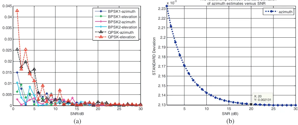
We increase the number of snapshots to 200, and the other conditions are the same as above. The results are shown in Fig. 6. Compared with Fig. 5, both the deviation and standard deviation are

0 5 10 15 20 25 30

0 0.005 0.01 0.015 0.02 0.025 0.03 0.035 0.04 0.045

SNR/dB

dev

ia

ti

on/

°

BPSK1-azimuth BPSK1-elevation BPSK2-azimuth BPSK2-elevation QPSK-azimuth QPSK-elevation

5 10 15 20 25 30

2.13 2.14 2.15 2.16 2.17 2.18 2.19 2.2 2.21 2.22 2.23

x 10-3

X: 20 Y: 0.002131

SNR (dB)

S

T

A

NDA

RD Dev

ia

ti

o

n

The relationship between Standard Deviation of azimuth estimates versus SNR

azimuth

(a) (b)

Figure 6. The performance of the MS-MUSIC withK = 200. (a) Deviation of estimates versus SNR. (b) Standard Deviation of estimates versus SNR.

0 100 200 300 400 500 600 700 800 900 1000 0

0.005 0.01 0.015 0.02 0.025 0.03

number of snapshots

S

T

A

NDA

RD Dev

ia

ti

o

n

STANDARD Deviation versus number of snapshots

MS-MUSIC Maximum Likelihood Traditional MUSIC

improved, which is expected. Obviously, in the engineering design, the more the snapshots are, the better estimation performance we can obtain. If we choose the point where the SNR equals 20 dB, we can find the standard deviations of the two cases as 0.0042 (K = 100) and 0.0021 (K = 200), respectively. In fact, these improvements can be predicted from Formula (31). In Formula (31), the number of snapshots can be extracted from the Fisher information matrix. Moreover, the CRLB is found as the [i, j] element of the inverse of the I(θ). So, we can conclude that CRLB is inversely proportional toK. Thus, the estimation precision will be higher. The simulation results also verify the validity of the MS-MUSIC algorithm.

Figure 7 shows the standard deviation versus the number of snapshots of the MS-MUSIC, traditional MUSIC and the maximum likelihood. Similarly, the standard deviation is considered as the mean of the azimuth angles of the mixed signals. The SNR is fixed at 20 dB. The performances of the three algorithms are improved with the increase of number of snapshots. The proposed algorithm outperforms the other two methods in the entire range especially when the number of snapshots is small. The reason is that we exploit the extra information (i.e., the conjugate correlation statistical information) of the non-circular signals.

6. CONCLUSION

For mixed non-circular and circular signals co-incident problems, the array output signal model based on a circular array is analyzed, and the MS-MUSIC algorithm is proposed. On this basis, we derive the CRLB. Compared with the existing methods, the proposed one has two main advantages. Firstly, it acquires higher estimation accuracy by exploiting the conjugate relation characteristics. Secondly, the circular signals can be identified easily which decreases the computational burden. Monte-Carlo simulation results are presented verifying the efficacy of the proposed algorithm.

ACKNOWLEDGMENT

This project was supported by the National Natural Science Foundation of China (Grant No. 61302017). The authors would like to thank the anonymous reviewers for the improvement of this paper.

REFERENCES

1. Xu, Y. and Z. Liu, “Noncircularity-exploitation in direction estimation of noncircular signals with an acoustic vector-sensor,” Digital Signal Processing, Vol. 18, 777–796, 2008, ISSN: 1051-2004, DOI: 10.1016/j.dsp.2007.10.008.

2. Longstaff, I. D., P. E. K. Chow, et al., “Directional properties of circular arrays,” IEE Proc., Vol. 114, No. 6, 713–718, 1967, DOI: 10.1049/piee.1967.0142.

3. Mathews, C. P. and M. D. Zoltowski, “Eigenstructure techniques for 2-D angle estimation with uniform circular arrays,”IEEE Transactions on Signal Processing, Vol. 42, No. 9, 2395–2407, 1994, ISSN: 1053-587X, DOI: 10.1109/78.317861

4. Abeida, H. and J. P. Delmas, “MUSIC-like estimation of direction of arrival for noncircular sources,”

IEEE Transactions on Signal Processing, Vol. 54, No. 7, 2678–2690, 2006, ISSN: 1053-587X,

DOI: 10.1109/TSP.2006.873505.

5. Guo, R., X.-P. Mao, S.-B. Li, Y.-M. Wang, and X.-H. Wang, “A fast DOA estimation algorithm based on polarization MUSIC,” Radioengineering, Vol. 24, No. 1, 214–225, 2015, DOI: 10.13164/re.2015.0214.

6. Shi, Y., L. Huang, C. Qian, and H. C. So, “Direction-of-Arrival estimation for noncircular sources via structured least squares-based ESPRIT using three-axis crossed array,” IEEE Transactions on Aerospace and Electroninc Systems, Vol. 51, No. 2, 1267–1278, 2015, ISSN: 0018-9251, DOI: 10.1109/TAES.2015.140003.

8. Tomic, S., M. Beko, and R. Dinis, “Distributed RSS-AoA based localization with unknown transmit powers,” IEEE Wireless Communications Letters, Vol. PP, No. 99, 1–1, 2016, DOI: 10.1109/LWC.2016.2567394.

9. Li, J. and R. T. Compton, “Angle estimation using a polarization sensitive array,” IEEE Transactions on Antennas and Propagation, Vol. 39, No. 10, 1539–1543, 1991, ISSN: 0018-926X, DOI:10.1109/8.97389.

10. Deschamps, G. A., “Techniques for handling elliptically polarized waves with special reference to antennas: Part II — Geometrical representation of the polarization of a plane electromagnetic wave,” Proceedings of the I.R.E., Vol. 39, 540–544, 1951, DOI:10.1109/JRPROC.1951.233136. 11. Nehorai, A. and E. Paldi, “Vector-sensor array processing for electromagnetic source localization,”

IEEE Transactions on Signal Processing, Vol. 42, No. 2, 376–398, 1994, ISSN: 1053-587/94,

DOI: 10.1109/78.275610.

12. Schmidt, R., “Multiple emitter location and signal parameter estimation,” IEEE

Trans-actions on Antennas and Propagation, Vol. 34, No. 3, 276–280, 1986, ISSN: 0018-926X,

DOI: 10.1109/TAP.1986.1143830.

13. Bellman, R., Introduction to Matrix Analysis, 2nd Edition, The RAND Corporation, New York, USA, 1997, ISBN: 0-89871-3994.

14. Stoica, P. and A. Nehorai, “MUSIC, maximum likelihood, and Cramer-Rao bound,” IEEE Transactions on Acoustics Speech and Signal Processing, Vol. 37, No. 5, 720–741, ISSN: 0096-3518, DOI: 10.1109/29.17564, 1989.

15. Stoica, P. and A. Nehorai, “MUSIC, maximum likelihood, and Cramer-Rao bound: Further results and comparisons,” IEEE Transactions on Acoustics SPEFCH and Signal Processing, Vol. 38, No. 12, 2140–2150, 1990, ISSN: 0096-3518, DOI: 10.1109/29.61541.